Background Estimation (photutils.background)#
Introduction#
To accurately measure the photometry and morphological properties of astronomical sources, one requires an accurate estimate of the background, which can be from both the sky and the detector. Similarly, having an accurate estimate of the background noise is important for determining the significance of source detections and for estimating photometric errors.
Unfortunately, accurate background and background noise estimation is a difficult task. Further, because astronomical images can cover a wide variety of scenes, there is not a single background estimation method that will always be applicable. Photutils provides tools for estimating the background and background noise in your data, but they will likely require some tweaking to optimize the background estimate for your data.
Scalar Background and Noise Estimation#
Simple Statistics#
If the background level and noise are relatively constant across an image, the simplest way to estimate these values is to derive scalar quantities using simple approximations. When computing the image statistics one must take into account the astronomical sources present in the images, which add a positive tail to the distribution of pixel intensities. For example, one may consider using the image median as the background level and the image standard deviation as the 1-sigma background noise, but the resulting values are biased by the presence of real sources.
A slightly better method involves using statistics that are robust against the presence of outliers, such as the biweight location for the background level and biweight scale or normalized median absolute deviation (MAD) for the background noise estimation. However, for most astronomical scenes these methods will also be biased by the presence of astronomical sources in the image.
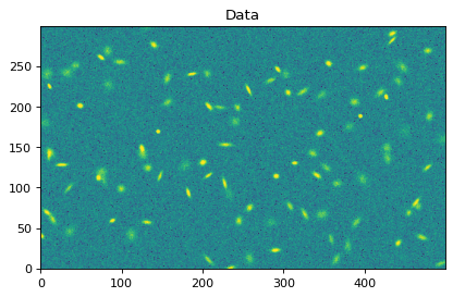
As an example, we load a synthetic image comprised of 100 sources with a Gaussian-distributed background whose mean is 5 and standard deviation is 2:
>>> from photutils.datasets import make_100gaussians_image
>>> data = make_100gaussians_image()
Let’s plot the image:
>>> import matplotlib.pyplot as plt
>>> from astropy.visualization import simple_norm
>>> norm = simple_norm(data, 'sqrt', percent=99.5)
>>> fig, ax = plt.subplots()
>>> ax.imshow(data, norm=norm, origin='lower')
(Source code, png, hires.png, pdf, svg)
The image median and biweight location are both larger than the true background level of 5:
>>> import numpy as np
>>> from astropy.stats import biweight_location
>>> print(np.median(data))
5.222396450477202
>>> print(biweight_location(data))
5.187556942771537
Similarly, using the median absolute deviation to estimate the background noise level gives a value that is larger than the true value of 2:
>>> from astropy.stats import mad_std
>>> print(mad_std(data))
2.1497096320053166
Sigma Clipping Sources#
The most widely used technique to remove the sources from the image statistics is called sigma clipping. Briefly, pixels that are above or below a specified sigma level from the median are discarded and the statistics are recalculated. The procedure is typically repeated over a number of iterations or until convergence is reached. This method provides a better estimate of the background and background noise levels:
>>> from astropy.stats import sigma_clipped_stats
>>> mean, median, std = sigma_clipped_stats(data, sigma=3.0)
>>> print(np.array((mean, median, std)))
[5.19968673 5.15244174 2.09423739]
Masking Sources#
An even better procedure is to exclude the sources in the image by masking them. This technique requires one to identify the sources in the data, which in turn depends on the background and background noise. Therefore, this method for estimating the background and background RMS requires an iterative procedure.
One method to create a source mask is to use a
segmentation image. Here we use the
detect_threshold convenience function to get a
rough estimate of the threshold at the 2-sigma background noise level.
Then we use the detect_sources function to
generate a SegmentationImage. Finally, we use
the make_source_mask()
method with a circular dilation footprint to create the source mask:
>>> from astropy.stats import sigma_clipped_stats, SigmaClip
>>> from photutils.segmentation import detect_threshold, detect_sources
>>> from photutils.utils import circular_footprint
>>> sigma_clip = SigmaClip(sigma=3.0, maxiters=10)
>>> threshold = detect_threshold(data, n_sigma=2.0, sigma_clip=sigma_clip)
>>> segment_img = detect_sources(data, threshold, n_pixels=10)
>>> footprint = circular_footprint(radius=10)
>>> mask = segment_img.make_source_mask(footprint=footprint)
>>> mean, median, std = sigma_clipped_stats(data, sigma=3.0, mask=mask)
>>> print(np.array((mean, median, std)))
[5.00257401 4.99641799 1.97009566]
The source detection and masking procedure can be iterated further. Even with one iteration we are within 0.2% of the true background value and 1.5% of the true background RMS.
2D Background and Noise Estimation#
If the background or the background noise varies across the image, then you will generally want to generate a 2D image of the background and background RMS (or compute these values locally). This can be accomplished by applying the above techniques to subregions of the image. A common procedure is to use sigma-clipped statistics in each mesh of a grid that covers the input data to create a low-resolution background image. The final background or background RMS image can then be generated by interpolating the low-resolution image.
Photutils provides the Background2D
class to estimate the 2D background and background noise in an
astronomical image. Background2D
requires the size of the box (box_size) in which to estimate the
background. Selecting the box size requires some care by the user.
The box size should generally be larger than the typical size of
sources in the image, but small enough to encapsulate any background
variations. For best results, the box size should also be chosen so
that the data are covered by an integer number of boxes in both
dimensions. If that is not the case, the image will be padded along
the top and/or right edges.
The background level in each of the meshes is calculated using
the function or callable object (e.g., class instance) input via
bkg_estimator keyword. Photutils provides several background
classes that can be used:
The default is a SExtractorBackground instance.
For this method, the background in each mesh is calculated as (2.5 *
median) - (1.5 * mean). However, if (mean - median) / std > 0.3
then the median is used instead.
Likewise, the background RMS level in each mesh is calculated using the
function or callable object input via the bkg_rms_estimator keyword.
Photutils provides the following classes for this purpose:
For even more flexibility, users may input a custom function or callable
object to the bkg_estimator and/or bkg_rms_estimator keywords.
By default, the bkg_estimator and bkg_rms_estimator are
applied to sigma clipped data. Sigma clipping is defined by inputting
a astropy.stats.SigmaClip object to the sigma_clip
keyword. The default is to perform sigma clipping with sigma=3
and maxiters=10. Sigma clipping can be turned off by setting
sigma_clip=None.
After the background level has been determined in each of the boxes, the
low-resolution background image can be median filtered, with a window
of size of filter_size, to suppress local under or over estimations
(e.g., due to bright galaxies in a particular box). Likewise, the median
filter can be applied only to those boxes where the background level is
above a specified threshold (filter_threshold).
The low-resolution background and background RMS images are resized to
the original data size using spline interpolation via
scipy.ndimage.zoom.
Note
Prior to version 3.0, the interpolation method could
be customized via the interpolator keyword using
BkgZoomInterpolator or
BkgIDWInterpolator classes. These
are now deprecated. The BkgIDWInterpolator is not well-suited
for resizing images on a regular grid to larger sizes. It is
also significantly slower than the default interpolator based on
scipy.ndimage.zoom.
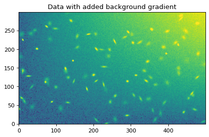
For this example, we will create a test image by adding a strong background gradient to the image defined above:
>>> ny, nx = data.shape
>>> y, x = np.mgrid[:ny, :nx]
>>> gradient = x * y / 5000.0
>>> data2 = data + gradient
>>> fig, ax = plt.subplots()
>>> ax.imshow(data2, norm=norm, origin='lower')
(Source code, png, hires.png, pdf, svg)
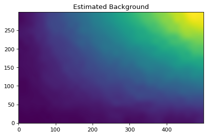
We start by creating a Background2D object
using a box size of 15x15 and a 3x3 median filter. We will estimate
the background level in each mesh as the sigma-clipped median using an
instance of MedianBackground:
>>> from astropy.stats import SigmaClip
>>> from photutils.background import Background2D, MedianBackground
>>> sigma_clip = SigmaClip(sigma=3.0)
>>> bkg_estimator = MedianBackground()
>>> bkg = Background2D(data2, (15, 15), filter_size=(3, 3),
...                    sigma_clip=sigma_clip, bkg_estimator=bkg_estimator)
The 2D background and background RMS images are retrieved using the
background and background_rms attributes, respectively, on the
returned object. The low-resolution versions of these images are stored
in the background_mesh and background_rms_mesh attributes,
respectively. The global median value of the low-resolution background
and background RMS image can be accessed with the background_median
and background_rms_median attributes, respectively:
>>> print(bkg.background_median)
10.822232525276007
>>> print(round(bkg.background_rms_median, 4))
2.0367
Let’s plot the background image:
>>> fig, ax = plt.subplots()
>>> ax.imshow(bkg.background, origin='lower')
(Source code, png, hires.png, pdf, svg)
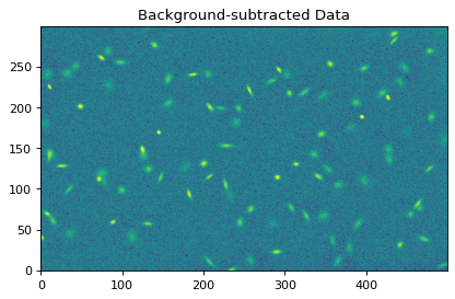
and the background-subtracted image:
>>> data2_sub = data2 - bkg.background
>>> fig, ax = plt.subplots()
>>> ax.imshow(data2_sub, norm=norm, origin='lower')
(Source code, png, hires.png, pdf, svg)
Masking#
Masks can also be input into Background2D. The
mask keyword can be used to mask sources or bad pixels in the image
prior to estimating the background levels.
Additionally, the coverage_mask keyword can be used to mask blank
regions without data coverage (e.g., from a rotated image or an image
from a mosaic). Otherwise, the data values in the regions without
coverage (usually zeros or NaNs) will adversely affect the background
statistics. Unlike mask, coverage_mask is applied to the output
background and background RMS maps. The fill_value keyword defines
the value assigned in the output background and background RMS maps
where the input coverage_mask is True.
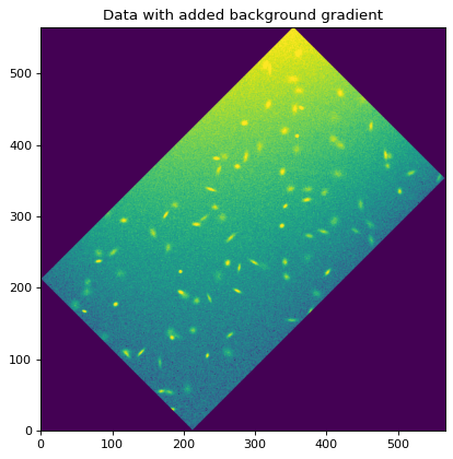
Let’s create a rotated image that has blank areas and plot it:
>>> from astropy.visualization import simple_norm
>>> from scipy.ndimage import rotate
>>> data3 = rotate(data2, -45.0)
>>> norm = simple_norm(data3, 'sqrt', percent=99.5)
>>> fig, ax = plt.subplots()
>>> ax.imshow(data3, norm=norm, origin='lower')
(Source code, png, hires.png, pdf, svg)
Now we create a coverage mask and input it into
Background2D to exclude the regions where we
have no data. For this example, we set the fill_value to 0.0. For
real data, one can usually create a coverage mask from a weight or noise
image. In this example we also use a smaller box size to help capture
the strong gradient in the background. We also increase the value of the
exclude_percentile keyword to include more boxes around the edge of
the rotated image:
>>> coverage_mask = (data3 == 0)
>>> bkg3 = Background2D(data3, (15, 15), filter_size=(3, 3),
...                     coverage_mask=coverage_mask, fill_value=0.0,
...                     exclude_percentile=50.0)
Note that the coverage_mask is applied to the output background
image (values assigned to fill_value):
>>> norm = simple_norm(bkg3.background, 'sqrt', percent=99.5)
>>> fig, ax = plt.subplots()
>>> ax.imshow(bkg3.background, norm=norm, origin='lower')
(Source code, png, hires.png, pdf, svg)

Finally, let’s subtract the background from the image and plot it:
>>> norm = ImageNormalize(stretch=SqrtStretch())
>>> data_sub = data3 - bkg3.background
>>> norm = simple_norm(data_sub, 'sqrt', percent=99.5)
>>> fig, ax = plt.subplots()
>>> ax.imshow(data_sub, norm=norm, origin='lower')
(Source code, png, hires.png, pdf, svg)
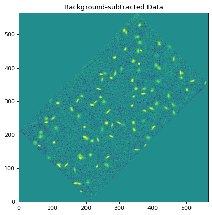
If there is any small residual background still present in the image, the background subtraction can be improved by masking the sources and/or through further iterations.
Plotting Meshes#
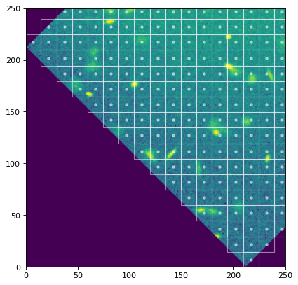
Finally, the meshes that were used in generating the 2D
background can be plotted on the original image using the
plot_meshes() method. Here we
zoom in on a small portion of the image to show the background meshes.
Meshes without a center marker were excluded.
>>> fig, ax = plt.subplots()
>>> ax.imshow(data3, norm=norm, origin='lower')
>>> bkg3.plot_meshes(outlines=True, marker='.', color='cyan', alpha=0.3)
>>> ax.set_xlim(0, 250)
>>> ax.set_ylim(0, 250)
(Source code, png, hires.png, pdf, svg)