Source Grouping#
Introduction#
In Point Spread Function (PSF) photometry, the accuracy of measuring a source’s brightness can be compromised by the light from nearby sources. When sources are close to each other, their individual light profiles overlap, affecting the fit of the PSF model used for measurement. To address this, a grouping algorithm can be employed to combine neighboring sources into distinct sets that are then analyzed simultaneously.
The primary objective of this grouping is to ensure that the light from any source within one group does not significantly spill over into the area where a source in another group is being measured. This method of creating and analyzing smaller groups of sources is more computationally efficient than attempting to fit a model to all the sources in an image at once, a task that is often impractical, especially in densely populated star fields.
A straightforward method for this grouping was introduced by Stetson (1987). This algorithm determines whether a given source’s light profile interferes with that of any other source by using a “critical separation” parameter. This parameter sets the minimum distance required between two source for them to be placed in separate groups. Typically, this critical separation is defined as a multiple of the stellar full width at half maximum (FWHM), which is a measure of the source’s apparent size.
Getting Started#
To group sources, Photutils includes a tool called
SourceGrouper. This class organizes sources
into groups by applying a technique known as hierarchical agglomerative
clustering, which uses a distance-based criterion. This functionality is
implemented using the scipy.cluster.hierarchy.fclusterdata function
from the SciPy library.
Typically, to group sources during PSF fitting, one would provide a
SourceGrouper object, configured with a minimum
separation distance, directly to one of the PSF photometry classes.
However, for the purpose of illustration, we will show how to use the
SourceGrouper class independently to group stars
within a sample image.
The first step is to generate a simulated astronomical image that
contains sources modeled as 2D Gaussians, which we will accomplish using
the make_psf_model_image function:
>>> from photutils.datasets import make_noise_image
>>> from photutils.psf import CircularGaussianPRF, make_psf_model_image
>>> shape = (256, 256)
>>> fwhm = 4.7
>>> psf_model = CircularGaussianPRF(fwhm=fwhm)
>>> psf_shape = (11, 11)
>>> n_sources = 100
>>> flux = (500, 1000)
>>> border_size = (7, 7)
>>> data, stars = make_psf_model_image(shape, psf_model, n_sources,
...                                    model_shape=psf_shape,
...                                    flux=flux,
...                                    border_size=border_size, seed=123)
>>> noise = make_noise_image(shape, mean=0, stddev=2, seed=123)
>>> data += noise
The make_psf_model_image provides two outputs: the
image itself, which we call data, and a table containing the
positions and fluxes of the stars, which we call stars. The x and y
coordinates of the stars are located in the x_0 and y_0 columns
of this table.
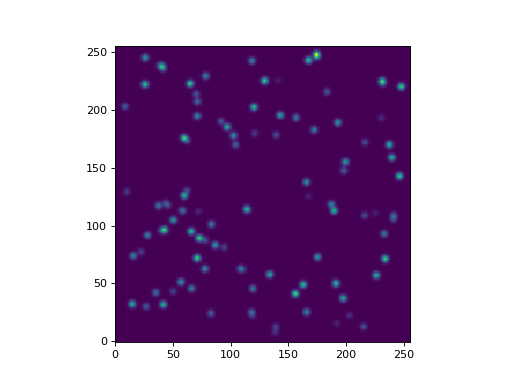
Let’s display the image:
>>> import matplotlib.pyplot as plt
>>> fig, ax = plt.subplots(figsize=(8, 8))
>>> ax.imshow(data, origin='lower')
(Source code, png, hires.png, pdf, svg)


With the simulated data ready, we can now identify groups of stars.
The first step is to create a SourceGrouper object.
For this example, we will define the minimum separation between stars
in different groups (min_separation) as 2.5 times the full width
at half maximum (FWHM). The FWHM value is known because it was used to
create the simulated stars. In a real-world scenario, you would first
need to measure the FWHM from the actual star images:
>>> from photutils.psf import SourceGrouper
>>> fwhm = 4.7
>>> min_separation = 2.5 * fwhm
>>> grouper = SourceGrouper(min_separation)
After initializing the SourceGrouper, we apply it to
the x and y coordinates of the stars. While we are using the known, true
positions from our simulated data, you would typically use a source
detection tool to find the star positions in an actual image:
>>> import numpy as np
>>> x = np.array(stars['x_0'])
>>> y = np.array(stars['y_0'])
>>> group_ids = grouper(x, y)
>>> print(group_ids[:20])  # first 20 group IDs
[ 1  2  3  4  5  6  7  8  9 10 11  4  6  3 12 13 14 15 16 17]
The result of this process is an array of integers, group_id, where
each integer represents the group to which the corresponding star.
Stars that share the same group ID are considered part of the same
group.
When performing PSF photometry, you can add the group IDs to the initial
parameters table (init_params) that is passed to the photometry
tool. If you provide these group IDs, a SourceGrouper
does not need to be passed to the photometry class, as the grouping will
already be defined.
Returning a SourceGroups Object#
Alternatively, you can set the return_groups_object keyword to
True when calling the SourceGrouper object, and
it will return a SourceGroups object instead of an
array of integers:
>>> groups = grouper(x, y, return_groups_object=True)
>>> print(type(groups))
<class 'photutils.psf.groupers.SourceGroups'>
In this case, groups is a SourceGroups object
that contains the grouping results and provides convenient methods for
analysis. This object stores the source coordinates, group IDs, and
provides properties and methods to analyze the grouping.
The grouping algorithm separated the 100 stars into 65 distinct groups:
>>> print(groups.n_groups)
65
You can access the group IDs directly from the groups attribute,
which is an array of integers corresponding to the input star
coordinates. Stars with the same group ID belong to the same group:
>>> print(groups.groups[:20])  # first 20 group IDs
[ 1  2  3  4  5  6  7  8  9 10 11  4  6  3 12 13 14 15 16 17]
Similar to above, you can add the group IDs from groups.groups to
the initial parameters table (init_params) that is passed to the
photometry tool to define the source grouping.
To find the positions of the stars in group 3, you can use the
get_group_sources method:
>>> x_group3, y_group3 = groups.get_group_sources(3)
>>> print(x_group3, y_group3)
[60.32708921 58.73063714] [147.24184586 158.0612346 ]
The SourceGroups object also provides useful properties
and methods to analyze the grouping results:
>>> # Get the size of each group for each source
>>> sizes = groups.sizes
>>> print(f'Group sizes: {sizes[:5]}')  # first 5
Group sizes: [1 2 2 5 2]

>>> # Get the mapping of group IDs to group sizes
>>> size_map = groups.size_map
>>> print(f'Size map: {list(size_map.items())[:5]}')  # first 5
Size map: [(1, 1), (2, 2), (3, 2), (4, 5), (5, 2)]

>>> print(f'Largest group size: {max(size_map.values())}')
Largest group size: 5

>>> # Get a list of group IDs that have the largest group size
>>> largest_group_ids = ([gid for gid, size in size_map.items()
...                       if size == max(size_map.values())])
>>> print(f'Largest group IDs: {largest_group_ids}')
Largest group IDs: [4]

>>> # Get the centroid of group 5
>>> xy_center = groups.group_centers[5]
>>> print(f'Group 5 center: {xy_center}')
Group 5 center: (48.35899721341876, 73.85258893310564)
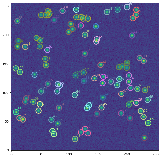
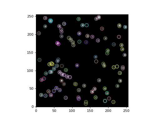
To visualize the results, we can use the
plot method, which draws color-coded
circles around each star to show which stars have been grouped together:
>>> import matplotlib.pyplot as plt
>>> fig, ax = plt.subplots(figsize=(8, 8))
>>> ax.imshow(data, origin='lower')
>>> groups.plot(radius=fwhm, ax=ax, lw=2, seed=123)
(Source code, png, hires.png, pdf, svg)


You can also label each group with its ID by setting the label_groups
keyword:
>>> import matplotlib.pyplot as plt
>>> fig, ax = plt.subplots(figsize=(8, 8))
>>> ax.imshow(data, origin='lower')
>>> groups.plot(radius=fwhm, ax=ax, lw=2, seed=123,
                label_groups=True, label_offset=(6, 6))
(Source code, png, hires.png, pdf, svg)