Aperture Photometry (`photutils.aperture`)#

Introduction#

The aperture_photometry() function and the ApertureStats class are the main tools to perform aperture photometry on an astronomical image for a given set of apertures.

Apertures#

Photutils provides several apertures defined in pixel or sky coordinates. The aperture classes that are defined in pixel coordinates are:

Each of these classes has a corresponding variant defined in sky coordinates:

To perform aperture photometry with sky-based apertures, one will need to specify a WCS transformation.

The aperture_photometry() function and the ApertureStats class both accept Aperture objects. They can also accept a supported regions.Region object, i.e. a region that corresponds to the above aperture classes, as input. The aperture_photometry() function also accepts a list of Aperture or regions.Region objects if each aperture/region has identical positions.

The region_to_aperture() convenience function can also be used to convert a regions.Region object to a Aperture object.

Users can also create their own custom apertures (see Defining Your Own Custom Apertures).

Creating Aperture Objects#

The first step in performing aperture photometry is to create an aperture object. An aperture object is defined by a position (or a list of positions) and parameters that define its size and possibly, orientation (e.g., an elliptical aperture).

We start with an example of creating a circular aperture in pixel coordinates using the CircularAperture class:

>>> from photutils.aperture import CircularAperture
>>> positions = [(30.0, 30.0), (40.0, 40.0)]
>>> aperture = CircularAperture(positions, r=3.0)

The positions should be either a single tuple of (x, y), a list of (x, y) tuples, or an array with shape Nx2, where N is the number of positions. The above example defines two circular apertures located at pixel coordinates (30, 30) and (40, 40) with a radius of 3 pixels.

Creating an aperture object in sky coordinates is similar. One first uses the SkyCoord class to define sky coordinates and then the SkyCircularAperture class to define the aperture object:

>>> from astropy import units as u
>>> from astropy.coordinates import SkyCoord
>>> from photutils.aperture import SkyCircularAperture
>>> positions = SkyCoord(l=[1.2, 2.3] * u.deg, b=[0.1, 0.2] * u.deg,
...                      frame='galactic')
>>> aperture = SkyCircularAperture(positions, r=4.0 * u.arcsec)

Note

Sky apertures are not defined completely in sky coordinates. They simply use sky coordinates to define the central position, and the remaining parameters are converted to pixels using the pixel scale of the image at the central position. Projection distortions are not taken into account. They are not defined as apertures on the celestial sphere, but rather are meant to represent aperture shapes on an image. If the apertures were defined completely in sky coordinates, their shapes would not be preserved when converting to or from pixel coordinates.

Converting Between Pixel and Sky Apertures#

The pixel apertures can be converted to sky apertures, and vice versa, given a WCS object. To accomplish this, use the to_sky() method for pixel apertures. For this example, we’ll use a sample WCS object:

>>> from photutils.datasets import make_wcs
>>> wcs = make_wcs((100, 100))
>>> aperture = CircularAperture((10, 20), r=4.0)
>>> sky_aperture = aperture.to_sky(wcs)
>>> sky_aperture  
<SkyCircularAperture(<SkyCoord (ICRS): (ra, dec) in deg
    (197.89234399, -1.36689653)>, r=0.39999999985539925 arcsec)>

and the to_pixel() method for sky apertures, e.g.,:

>>> position = SkyCoord(197.893, -1.366, unit='deg', frame='icrs')
>>> aperture = SkyCircularAperture(position, r=0.4 * u.arcsec)
>>> pix_aperture = aperture.to_pixel(wcs)
>>> pix_aperture  
<CircularAperture([26.14628817, 56.58410628], r=4.000000000439743)>

Performing Aperture Photometry#

After the aperture object is created, we can then perform the photometry using the aperture_photometry() function. We start by defining the aperture (at two positions) as described above:

>>> positions = [(30.0, 30.0), (40.0, 40.0)]
>>> aperture = CircularAperture(positions, r=3.0)

We then call the aperture_photometry() function with the data and the apertures. Note that aperture_photometry() assumes that the input data have been background subtracted. For simplicity, we define the data here as an array of all ones:

>>> import numpy as np
>>> from photutils.aperture import aperture_photometry
>>> data = np.ones((100, 100))
>>> phot_table = aperture_photometry(data, aperture)
>>> phot_table['aperture_sum'].info.format = '%.8g'  # for consistent table output
>>> print(phot_table)
 id xcenter ycenter aperture_sum
--- ------- ------- ------------
  1    30.0    30.0    28.274334
  2    40.0    40.0    28.274334

This function returns the results of the photometry in an Astropy QTable. In this example, the table has four columns, named 'id', 'xcenter', 'ycenter', and 'aperture_sum'.

Since all the data values are 1.0, the aperture sums are equal to the area of a circle with a radius of 3:

>>> print(np.pi * 3.0 ** 2)  
28.2743338823

Aperture and Pixel Overlap#

The overlap of the aperture with the data pixels can be handled in different ways. The default method (method='exact') calculates the exact intersection of the aperture with each pixel. The other options, 'center' and 'subpixel', are faster, but with the expense of less precision. With 'center', a pixel is considered to be entirely in or out of the aperture depending on whether its center is in or out of the aperture. With 'subpixel', pixels are divided into a number of subpixels, which are in or out of the aperture based on their centers. For this method, the number of subpixels needs to be set with the subpixels keyword.

This example uses the 'subpixel' method where pixels are resampled by a factor of 5 (subpixels=5) in each dimension:

>>> phot_table = aperture_photometry(data, aperture, method='subpixel',
...                                  subpixels=5)
>>> print(phot_table)  
 id xcenter ycenter aperture_sum
--- ------- ------- ------------
  1    30.0    30.0        27.96
  2    40.0    40.0        27.96

Note that the results differ from the exact value of 28.274333 (see above).

For the 'subpixel' method, the default value is subpixels=5, meaning that each pixel is equally divided into 25 smaller pixels (this is the method and subsampling factor used in SourceExtractor).

The precision can be increased by increasing subpixels, but note that computation time will be increased.

Aperture Photometry with Multiple Apertures at Each Position#

While the Aperture objects support multiple positions, they must have a fixed size and shape (e.g., radius and orientation).

To perform photometry in multiple apertures at each position, one may input a list of aperture objects to the aperture_photometry() function. In this case, the apertures must all have identical position(s).

Suppose that we wish to use three circular apertures, with radii of 3, 4, and 5 pixels, on each source:

>>> radii = [3.0, 4.0, 5.0]
>>> apertures = [CircularAperture(positions, r=r) for r in radii]
>>> phot_table = aperture_photometry(data, apertures)
>>> for col in phot_table.colnames:
...     phot_table[col].info.format = '%.8g'  # for consistent table output
>>> print(phot_table)
 id xcenter ycenter aperture_sum_0 aperture_sum_1 aperture_sum_2
--- ------- ------- -------------- -------------- --------------
  1      30      30      28.274334      50.265482      78.539816
  2      40      40      28.274334      50.265482      78.539816

For multiple apertures, the output table column names are appended with the positions index.

Other apertures have multiple parameters specifying the aperture size and orientation. For example, for elliptical apertures, one must specify a, b, and theta:

>>> from astropy.coordinates import Angle
>>> from photutils.aperture import EllipticalAperture
>>> a = 5.0
>>> b = 3.0
>>> theta = Angle(45, 'deg')
>>> apertures = EllipticalAperture(positions, a, b, theta)
>>> phot_table = aperture_photometry(data, apertures)
>>> for col in phot_table.colnames:
...     phot_table[col].info.format = '%.8g'  # for consistent table output
>>> print(phot_table)
 id xcenter ycenter aperture_sum
--- ------- ------- ------------
  1      30      30     47.12389
  2      40      40     47.12389

Again, for multiple apertures one should input a list of aperture objects, each with identical positions:

>>> a = [5.0, 6.0, 7.0]
>>> b = [3.0, 4.0, 5.0]
>>> theta = Angle(45, 'deg')
>>> apertures = [EllipticalAperture(positions, a=ai, b=bi, theta=theta)
...              for (ai, bi) in zip(a, b)]
>>> phot_table = aperture_photometry(data, apertures)
>>> for col in phot_table.colnames:
...     phot_table[col].info.format = '%.8g'  # for consistent table output
>>> print(phot_table)
 id xcenter ycenter aperture_sum_0 aperture_sum_1 aperture_sum_2
--- ------- ------- -------------- -------------- --------------
  1      30      30       47.12389      75.398224      109.95574
  2      40      40       47.12389      75.398224      109.95574

Aperture Statistics#

The ApertureStats class can be used to create a catalog of statistics and properties for pixels within an aperture, including aperture photometry. It can calculate many properties, including statistics like min, max, mean, median, std, sum_aper_area, and sum. It also can be used to calculate morphological properties like centroid, fwhm, semimajor_sigma, semiminor_sigma, orientation, and eccentricity. Please see ApertureStats for the complete list of properties that can be calculated. The properties can be accessed using ApertureStats attributes or output to an Astropy QTable using the to_table() method.

Most of the source properties are calculated using the “center” aperture-mask method, which gives aperture weights of 0 or 1. This avoids the need to compute weighted statistics — the data pixel values are directly used.

The sum_method and subpixels keywords are used to determine the aperture-mask method when calculating the sum-related properties: sum, sum_error, sum_aper_area, data_sumcutout, and error_sumcutout. The default is sum_method='exact', which produces exact aperture-weighted photometry.

The optional local_bkg keyword can be used to input the per-pixel local background of each source, which will be subtracted before computing the aperture statistics.

The optional sigma_clip keyword can be used to sigma clip the pixel values before computing the source properties. This keyword could be used, for example, to compute a sigma-clipped median of pixels in an annulus aperture to estimate the local background level.

Here is a simple example using a circular aperture at one position. Note that like aperture_photometry(), ApertureStats expects the input data to be background subtracted. For simplicity, here we roughly estimate the background as the sigma-clipped median value:

>>> from astropy.stats import sigma_clipped_stats
>>> from photutils.aperture import ApertureStats, CircularAperture
>>> from photutils.datasets import make_4gaussians_image

>>> data = make_4gaussians_image()
>>> _, median, _ = sigma_clipped_stats(data, sigma=3.0)
>>> data -= median  # subtract background from the data
>>> aper = CircularAperture((150, 25), 8)
>>> aperstats = ApertureStats(data, aper)  
>>> print(aperstats.xcentroid)  
149.98963482915323
>>> print(aperstats.ycentroid)  
24.97165265459083
>>> print(aperstats.centroid)  
[149.98963483  24.97165265]

>>> print(aperstats.mean, aperstats.median, aperstats.std)  
42.38192194155781 26.53270189818481 39.19365538349298

>>> print(aperstats.sum)  
8204.777345704442

Similar to aperture_photometry, the input aperture can have multiple positions:

>>> aper2 = CircularAperture(((150, 25), (90, 60)), 10)
>>> aperstats2 = ApertureStats(data, aper2)
>>> print(aperstats2.xcentroid)  
[149.98175939  89.97793821]
>>> print(aperstats2.sum)  
[ 8487.10695247 34963.45850824]
>>> columns = ('id', 'mean', 'median', 'std', 'var', 'sum')
>>> stats_table = aperstats2.to_table(columns)
>>> for col in stats_table.colnames:
...     stats_table[col].info.format = '%.8g'  # for consistent table output

>>> print(stats_table)  
 id    mean     median     std       var       sum
--- --------- --------- --------- --------- ---------
  1 27.915818 12.582676 36.628464 1341.6444  8487.107
  2 113.18737 112.11505 49.756626 2475.7218 34963.459

Each row of the table corresponds to a single aperture position (i.e., a single source).

Background Subtraction#

Global Background Subtraction#

aperture_photometry() and ApertureStats assume that the input data have been background-subtracted. If bkg is a float value or an array representing the background of the data (e.g., determined by Background2D or an external function), simply subtract the background from the data:

>>> phot_table = aperture_photometry(data - bkg, aperture)  

In the case of a constant global background, you can pass in the background value using local_bkg in ApertureStats. This would avoid reading an entire memory-mapped array into memory beforehand, as would happen if you manually subtract the background as shown above. So instead you could do this:

>>> aperstats = ApertureStats(data, aperture, local_bkg=bkg)  

Local Background Subtraction#

One often wants to also estimate the local background around each source using a nearby aperture or annulus aperture surrounding each source. A simple method for doing this is to use the ApertureStats class (see Aperture Statistics) to compute the mean background level within the background aperture. This class can also be used to calculate more advanced statistics (e.g., a sigma-clipped median) within the background aperture (e.g., a circular annulus). We show examples of both below.

Let’s start by generating a more realistic example dataset:

>>> from photutils.datasets import make_100gaussians_image
>>> data = make_100gaussians_image()

This artificial image has a known constant background level of 5. In the following examples, we’ll leave this global background in the image to be estimated using local backgrounds.

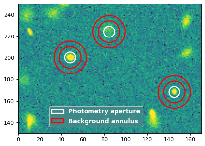
For this example we perform the photometry for three sources in a circular aperture with a radius of 5 pixels. The local background level around each source is estimated using a circular annulus of inner radius 10 pixels and outer radius 15 pixels. Let’s define the apertures:

>>> from photutils.aperture import CircularAnnulus, CircularAperture
>>> positions = [(145.1, 168.3), (84.5, 224.1), (48.3, 200.3)]
>>> aperture = CircularAperture(positions, r=5)
>>> annulus_aperture = CircularAnnulus(positions, r_in=10, r_out=15)

Now let’s plot the circular apertures (white) and circular annulus apertures (red) on a cutout from the image containing the three sources:

(Source code, png, hires.png, pdf, svg)

Simple mean within a circular annulus#

We can use the ApertureStats class to compute the mean background level within the annulus aperture at each position:

>>> from photutils.aperture import ApertureStats
>>> aperstats = ApertureStats(data, annulus_aperture)
>>> bkg_mean = aperstats.mean
>>> print(bkg_mean)  
[4.99411764 5.1349344  4.86894665]

Now let’s use aperture_photometry() to perform the photometry in the circular aperture (in the next example, we’ll use ApertureStats to perform the photometry):

>>> from photutils.aperture import aperture_photometry
>>> phot_table = aperture_photometry(data, aperture)
>>> for col in phot_table.colnames:
...     phot_table[col].info.format = '%.8g'  # for consistent table output
>>> print(phot_table)
 id xcenter ycenter aperture_sum
--- ------- ------- ------------
  1   145.1   168.3    1128.1245
  2    84.5   224.1      735.739
  3    48.3   200.3    1299.6341

The total background within the circular aperture is the mean local per-pixel background times the circular aperture area. If you are using the default “exact” aperture (see aperture-mask methods) and there are no masked pixels, the exact analytical aperture area can be accessed via the aperture area attribute:

>>> aperture.area  
78.53981633974483

However, in general you should use the photutils.aperture.PixelAperture.area_overlap() method where a mask keyword can be input. This ensures you are using the same area over which the photometry was performed. If using a SkyAperture, you will first need to convert it to a PixelAperture. Since we are not using a mask, the results are identical:

>>> aperture_area = aperture.area_overlap(data)
>>> print(aperture_area)  
[78.53981634 78.53981634 78.53981634]

The total background within the circular aperture is then:

>>> total_bkg = bkg_mean * aperture_area
>>> print(total_bkg)  
[392.23708187 403.29680431 382.40617574]

Thus, the background-subtracted photometry is:

>>> phot_bkgsub = phot_table['aperture_sum'] - total_bkg

Finally, let’s add these as columns to the photometry table:

>>> phot_table['total_bkg'] = total_bkg
>>> phot_table['aperture_sum_bkgsub'] = phot_bkgsub
>>> for col in phot_table.colnames:
...     phot_table[col].info.format = '%.8g'  # for consistent table output
>>> print(phot_table)
 id xcenter ycenter aperture_sum total_bkg aperture_sum_bkgsub
--- ------- ------- ------------ --------- -------------------
  1   145.1   168.3    1128.1245 392.23708           735.88739
  2    84.5   224.1      735.739  403.2968           332.44219
  3    48.3   200.3    1299.6341 382.40618           917.22792

Sigma-clipped median within a circular annulus#

For this example, the local background level around each source is estimated as the sigma-clipped median value within the circular annulus. We’ll use the ApertureStats class to compute both the photometry (aperture sum) and the background level:

>>> from astropy.stats import SigmaClip
>>> sigclip = SigmaClip(sigma=3.0, maxiters=10)
>>> aper_stats = ApertureStats(data, aperture, sigma_clip=None)
>>> bkg_stats = ApertureStats(data, annulus_aperture, sigma_clip=sigclip)

The sigma-clipped median values in the background annulus apertures are:

>>> print(bkg_stats.median)  
[4.89374178 5.05655328 4.83268958]

The total background within the circular apertures is then the per-pixel background level multiplied by the circular-aperture areas:

>>> total_bkg = bkg_stats.median * aper_stats.sum_aper_area.value
>>> print(total_bkg)  
[384.35358069 397.14076611 379.5585524 ]

Finally, the local background-subtracted sum within the circular apertures is:

>>> apersum_bkgsub = aper_stats.sum - total_bkg
>>> print(apersum_bkgsub)  
[743.77088731 338.59823118 920.07553956]

Note that if you want to compute all the source properties (i.e., in addition to only sum) on the local-background-subtracted data, you may input the per-pixel local background values to ApertureStats via the local_bkg keyword:

>>> aper_stats_bkgsub = ApertureStats(data, aperture,
...                                   local_bkg=bkg_stats.median)
>>> print(aper_stats_bkgsub.sum)  
[743.77088731 338.59823118 920.07553956]

Note these background-subtracted values are the same as those above.

Aperture Photometry Error Estimation#

If and only if the error keyword is input to aperture_photometry(), the returned table will include a 'aperture_sum_err' column in addition to 'aperture_sum'. 'aperture_sum_err' provides the propagated uncertainty associated with 'aperture_sum'.

For example, suppose we have previously calculated the error on each pixel value and saved it in the array error:

>>> positions = [(30.0, 30.0), (40.0, 40.0)]
>>> aperture = CircularAperture(positions, r=3.0)
>>> data = np.ones((100, 100))
>>> error = 0.1 * data

>>> phot_table = aperture_photometry(data, aperture, error=error)
>>> for col in phot_table.colnames:
...     phot_table[col].info.format = '%.8g'  # for consistent table output
>>> print(phot_table)
 id xcenter ycenter aperture_sum aperture_sum_err
--- ------- ------- ------------ ----------------
  1      30      30    28.274334       0.53173616
  2      40      40    28.274334       0.53173616

'aperture_sum_err' values are given by:

\[\Delta F = \sqrt{\sum_{i \in A} \sigma_{\mathrm{tot}, i}^2}\]

where \(A\) are the non-masked pixels in the aperture, and \(\sigma_{\mathrm{tot}, i}\) is the input error array.

In the example above, it is assumed that the error keyword specifies the total error — either it includes Poisson noise due to individual sources or such noise is irrelevant. However, it is often the case that one has calculated a smooth “background-only error” array, which by design doesn’t include increased noise on bright pixels. To include Poisson noise from the sources, we can use the calc_total_error() function.

Let’s assume we have a background-only image called bkg_error. If our data are in units of electrons/s, we would use the exposure time as the effective gain:

>>> from photutils.utils import calc_total_error
>>> effective_gain = 500  # seconds
>>> error = calc_total_error(data, bkg_error, effective_gain)  
>>> phot_table = aperture_photometry(data - bkg, aperture, error=error)  

Aperture Photometry with Pixel Masking#

Pixels can be ignored/excluded (e.g., bad pixels) from the aperture photometry by providing an image mask via the mask keyword:

>>> data = np.ones((5, 5))
>>> aperture = CircularAperture((2, 2), 2.0)
>>> mask = np.zeros(data.shape, dtype=bool)
>>> data[2, 2] = 100.0  # bad pixel
>>> mask[2, 2] = True
>>> t1 = aperture_photometry(data, aperture, mask=mask)
>>> t1['aperture_sum'].info.format = '%.8g'  # for consistent table output
>>> print(t1['aperture_sum'])
aperture_sum
------------
   11.566371

The result is very different if a mask image is not provided:

>>> t2 = aperture_photometry(data, aperture)
>>> t2['aperture_sum'].info.format = '%.8g'  # for consistent table output
>>> print(t2['aperture_sum'])
aperture_sum
------------
   111.56637

Aperture Photometry Using Sky Coordinates#

As mentioned in Creating Aperture Objects, performing photometry using apertures defined in sky coordinates simply requires defining a “sky” aperture at positions defined by a SkyCoord object. Here we show an example of photometry on real data using a SkyCircularAperture.

We start by loading a Spitzer 4.5 micron image of a region of the Galactic plane:

>>> import astropy.units as u
>>> from astropy.wcs import WCS
>>> from photutils.datasets import load_spitzer_catalog, load_spitzer_image
>>> hdu = load_spitzer_image()  
>>> data = u.Quantity(hdu.data, unit=hdu.header['BUNIT'])  
>>> wcs = WCS(hdu.header)  
>>> catalog = load_spitzer_catalog()  

The catalog contains (among other things) the Galactic coordinates of the sources in the image as well as the PSF-fitted fluxes from the official Spitzer data reduction. We define the apertures positions based on the existing catalog positions:

>>> positions = SkyCoord(catalog['l'], catalog['b'], frame='galactic')  
>>> aperture = SkyCircularAperture(positions, r=4.8 * u.arcsec)  

Now perform the photometry in these apertures on the data. The wcs object contains the WCS transformation of the image obtained from the FITS header. It includes the coordinate frame of the image and the projection from sky to pixel coordinates. The aperture_photometry function uses the WCS information to automatically convert the apertures defined in sky coordinates into pixel coordinates:

>>> phot_table = aperture_photometry(data, aperture, wcs=wcs)  

The Spitzer catalog also contains the official fluxes for the sources, so we can compare to our fluxes. Because the Spitzer catalog fluxes are in units of mJy and the data are in units of MJy/sr, we need to convert units before comparing the results. The image data have a pixel scale of 1.2 arcsec/pixel.

>>> import astropy.units as u
>>> factor = (1.2 * u.arcsec) ** 2 / u.pixel
>>> fluxes_catalog = catalog['f4_5']  
>>> converted_aperture_sum = (phot_table['aperture_sum'] *
...                           factor).to(u.mJy / u.pixel)  

Finally, we can plot the comparison of the photometry:

>>> import matplotlib.pyplot as plt
>>> plt.scatter(fluxes_catalog, converted_aperture_sum.value)
>>> plt.xlabel('Spitzer catalog PSF-fit fluxes ')
>>> plt.ylabel('Aperture photometry fluxes')

(Source code, png, hires.png, pdf, svg)

Despite using different methods, the two catalogs are in good agreement. The aperture photometry fluxes are based on a circular aperture with a radius of 4.8 arcsec. The Spitzer catalog fluxes were computed using PSF photometry. Therefore, differences are expected between the two measurements.

Aperture Masks#

All PixelAperture objects have a to_mask() method that returns a ApertureMask object (for a single aperture position) or a list of ApertureMask objects, one for each aperture position. The ApertureMask object contains a cutout of the aperture mask weights and a BoundingBox object that provides the bounding box where the mask is to be applied.

Let’s start by creating a circular-annulus aperture:

>>> from photutils.aperture import CircularAnnulus
>>> from photutils.datasets import make_100gaussians_image
>>> data = make_100gaussians_image()
>>> positions = [(145.1, 168.3), (84.5, 224.1), (48.3, 200.3)]
>>> aperture = CircularAnnulus(positions, r_in=10, r_out=15)

Now let’s create a list of ApertureMask objects using the to_mask() method using the aperture mask “exact” method:

>>> masks = aperture.to_mask(method='exact')

Let’s plot the first aperture mask:

>>> import matplotlib.pyplot as plt
>>> plt.imshow(masks[0])

(Source code, png, hires.png, pdf, svg)

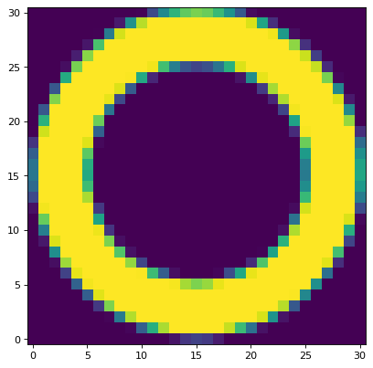
Let’s now use the “center” aperture mask method and plot the resulting aperture mask:

>>> masks2 = aperture.to_mask(method='center')
>>> plt.imshow(masks2[0])

(Source code, png, hires.png, pdf, svg)

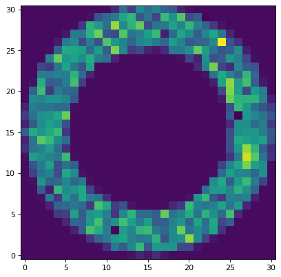
We can also create an aperture mask-weighted cutout from the data, properly handling the cases of partial or no overlap of the aperture mask with the data. Let’s plot the aperture mask weights (using the mask generated above with the “exact” method) multiplied with the data:

>>> data_weighted = masks[0].multiply(data)
>>> plt.imshow(data_weighted)

(Source code, png, hires.png, pdf, svg)

To get a 1D ndarray of the non-zero weighted data values, use the get_values() method:

>>> data_weighted_1d = masks[0].get_values(data)

The ApertureMask class also provides a to_image() method to obtain an image of the aperture mask in a 2D array of the given shape and a cutout() method to create a cutout from the input data over the aperture mask bounding box. Both of these methods properly handle the cases of partial or no overlap of the aperture mask with the data.

Defining Your Own Custom Apertures#

The aperture_photometry() function can perform aperture photometry in arbitrary apertures. This function accepts any Aperture-derived objects, such as CircularAperture. This makes it simple to extend functionality: a new type of aperture photometry simply requires the definition of a new Aperture subclass.

All PixelAperture subclasses must define a bounding_boxes property and to_mask() and plot() methods. They may also optionally define an area property. All SkyAperture subclasses must only implement a to_pixel() method.

bounding_boxes: The minimal bounding box for the aperture. If the aperture is scalar, then a single BoundingBox is returned. Otherwise, a list of BoundingBox is returned.
area: An optional property defining the exact analytical area (in pixels**2) of the aperture.
to_mask(): Return a mask for the aperture. If the aperture is scalar, then a single ApertureMask is returned. Otherwise, a list of ApertureMask is returned.
plot(): A method to plot the aperture on a matplotlib.axes.Axes instance.

API Reference#

Aperture Photometry (photutils.aperture)

Aperture Photometry (photutils.aperture)#

Introduction#

Apertures#

Creating Aperture Objects#

Converting Between Pixel and Sky Apertures#

Performing Aperture Photometry#

Aperture and Pixel Overlap#

Aperture Photometry with Multiple Apertures at Each Position#

Aperture Statistics#

Background Subtraction#

Global Background Subtraction#

Local Background Subtraction#

Simple mean within a circular annulus#

Sigma-clipped median within a circular annulus#

Aperture Photometry Error Estimation#

Aperture Photometry with Pixel Masking#

Aperture Photometry Using Sky Coordinates#

Aperture Masks#

Defining Your Own Custom Apertures#

API Reference#

Aperture Photometry (`photutils.aperture`)#