PSF Photometry (photutils.psf)#
The photutils.psf subpackage contains tools for model-fitting
photometry, often called “PSF photometry”.
Terminology#
Different astronomy subfields use the terms “PSF”, “PRF”, or related
terms in slightly varied ways, especially when colloquial usage is
taken into account. The photutils.psf package aims to be internally
consistent, following the definitions described here.
We take the Point Spread Function (PSF), or instrumental Point Spread Function (iPSF), to be the infinite-resolution and infinite-signal-to-noise flux distribution from a point source on the detector, after passing through optics, dust, atmosphere, etc. By contrast, the function describing the responsivity variations across individual pixels is the pixel response function. The pixel response function is sometimes called the “PRF”, but we do not use that acronym here to avoid confusion with the “Point Response Function” (see below). The convolution of the PSF and pixel response function, when discretized onto the detector (i.e., a rectilinear grid), is the effective PSF (ePSF) or Point Response Function (PRF). The PRF terminology is sometimes used to emphasize that the model function describes the response of the detector to a point source, rather than the intrinsic instrumental PSF (e.g., see the Spitzer Space Telescope MOPEX documentation).
In many cases the PSF/PRF/ePSF distinction is unimportant, and the PSF/PRF/ePSF is simply called the “PSF” model. However, the distinction can be critical when dealing carefully with undersampled data or detectors with significant intra-pixel sensitivity variations. For a more detailed description of this formalism, see Anderson & King 2000.
In colloquial usage, “PSF photometry” sometimes refers to the
more general task of model-fitting photometry with the effects of
the PSF either implicitly or explicitly included in the models,
regardless of exactly what kind of model is actually being fit. In the
photutils.psf package, we use “PSF photometry” in this way, as a
shorthand for the general approach.
PSF Photometry Overview#
Photutils provides a modular set of tools to perform PSF photometry for different science cases. The tools are implemented as classes that perform various subtasks of PSF photometry. High-level classes are also provided to connect these pieces together.
The two main PSF-photometry classes are PSFPhotometry
and IterativePSFPhotometry.
PSFPhotometry provides the framework for a flexible PSF
photometry workflow that can find sources in an image, optionally group
overlapping sources, fit the PSF model to the sources, and subtract the
fit PSF models from the image.
IterativePSFPhotometry is an iterative version of
PSFPhotometry where new sources are detected in the
residual image after the fit sources are subtracted. The iterative
process can be useful for crowded fields where sources are blended. A
mode keyword is provided to control the behavior of the iterative
process, where either all sources or only the newly-detected sources are
fit in subsequent iterations. The process repeats until no additional
sources are detected or a maximum number of iterations has been
reached. When used with the DAOStarFinder,
IterativePSFPhotometry is essentially an implementation
of the DAOPHOT algorithm described by Stetson in his seminal paper for
crowded-field stellar photometry.
The source-finding step is controlled by the finder
keyword, where one inputs a callable function or class
instance. Typically, this would be one of the source-detection
classes implemented in the photutils.detection
subpackage, e.g., DAOStarFinder,
IRAFStarFinder, or
StarFinder.
After finding sources, one can optionally apply a clustering algorithm
to group overlapping sources using the grouper keyword. Usually,
groups are formed by a distance criterion, which is the case of the
grouping algorithm proposed by Stetson. Sources that grouped are fit
simultaneously. The reason behind the construction of groups and not
fitting all sources simultaneously is illustrated as follows: imagine
that one would like to fit 300 sources and the model for each source
has three parameters to be fitted. If one constructs a single model to
fit the 300 sources simultaneously, then the optimization algorithm
will have to search for the solution in a 900-dimensional space, which
is computationally expensive and error-prone. Having smaller groups
of sources effectively reduces the dimension of the parameter space,
which facilitates the optimization process. For more details see
Source Grouping.
The local background around each source can optionally be subtracted
using the local_bkg_estimator keyword. This keyword accepts a
LocalBackground instance that estimates the
local statistics in a circular annulus aperture centered on each source.
The size of the annulus and the statistic function can be configured in
LocalBackground.
The next step is to fit the sources and/or groups. This
task is performed using an astropy fitter, for example
TRFLSQFitter, input via the fitter
keyword. The shape of the region to be fitted can be configured using
the fit_shape parameter. In general, fit_shape should be set to
a small size (e.g., (5, 5)) that covers the central part of the source
with the highest flux signal-to-noise. The initial positions are derived
from the finder algorithm. The initial flux values for the fit are
derived from measuring the flux in a circular aperture with radius
aperture_radius. Alternatively, the initial positions and fluxes can
be input in a table via the init_params keyword when calling the
class.
After sources are fitted, a model image of the fit
sources or a residual image can be generated using the
make_model_image() and
make_residual_image() methods,
respectively.
For IterativePSFPhotometry, the above steps can be
repeated until no additional sources are detected (or until a maximum
number of iterations is reached).
The PSFPhotometry and
IterativePSFPhotometry classes provide the structure
in which the PSF-fitting steps described above are performed, but
all the stages can be turned on or off or replaced with different
implementations as the user desires. This makes the tools very flexible.
One can also bypass several of the steps by directly inputting to
init_params an astropy table containing the initial parameters for
the source centers, fluxes, group identifiers, and local backgrounds.
This is also useful if one is interested in fitting only one or a few
sources in an image.
PSF Models#
As mentioned above, PSF photometry fundamentally involves fitting models to data. As such, the PSF model is a critical component of PSF photometry. For accurate results, both for photometry and astrometry, the PSF model should be a good representation of the actual data. The PSF model can be a simple analytic function, such as a 2D Gaussian or Moffat profile, or it can be a more complex model derived from a 2D PSF image, e.g., an effective PSF (ePSF). The PSF model can also encapsulate changes in the PSF across the detector, e.g., due to optical aberrations.
For image-based PSF models, the PSF model is typically derived from observed data or from detailed optical modeling. The PSF model can be a single PSF model for the entire image or a grid of PSF models at fiducial detector positions. Image-based PSF models are also often oversampled with respect to the pixel grid to increase the accuracy of fitting the PSF model.
The observatory that obtained the data may provide tools for creating
PSF models for their data or an empirical library of PSF models
based on previous observations. For example, the Hubble Space
Telescope provides libraries of
empirical PSF models for ACS and WFC3 (e.g., WFC3 PSF Search).
Similarly, the James Webb Space Telescope
and the Nancy Grace Roman Space Telescope
provide the STPSF Python software
for creating PSF models. In particular, WebbPSF outputs gridded PSF
models directly as Photutils GriddedPSFModel instances.
If you cannot obtain a PSF model from an empirical library or observatory-provided tool, Photutils provides tools for creating an empirical PSF model from the data itself, provided you have a large number of isolated stars. Please see Building an effective Point Spread Function (ePSF) for more information and an example.
The photutils.psf subpackage provides several PSF models that
can be used for PSF photometry. The PSF models are based on the
Astropy models and fitting framework.
The PSF models are used as input (via the psf_model parameter)
to the PSF photometry classes PSFPhotometry and
IterativePSFPhotometry. The PSF models are fitted to
the data using an Astropy fitter class. Typically, the model position
(x_0 and y_0) and flux (flux) parameters are varied
during the fitting process. The PSF model can also include additional
parameters, such as the full width at half maximum (FWHM) or sigma of
a Gaussian PSF or the alpha and beta parameters of a Moffat PSF. By
default, these additional parameters are “fixed” (i.e., not varied
during the fitting process). The user can choose to also vary these
parameters by setting the fixed attribute on the model parameter
to False. The position and/or flux parameters can also be fixed
during the fitting process if needed, e.g., for forced photometry (see
Forced Photometry (Fixed Model Parameters)). Any of the model parameters can also be
bounded during the fitting process (see Bounded Model Parameters).
You can also create your own custom PSF model using the Astropy modeling
framework. The PSF model must be a 2D model that is a subclass of
Fittable2DModel. It must have parameters called
x_0, y_0, and flux, specifying the central position and
total integrated flux.
Analytic PSF Models#
The photutils.psf subpackage provides the following analytic PSF
models:
GaussianPSF: a general 2D Gaussian PSF model parameterized in terms of the position, total flux, and full width at half maximum (FWHM) along the x and y axes. Rotation can also be included.CircularGaussianPSF: a circular 2D Gaussian PSF model parameterized in terms of the position, total flux, and FWHM.GaussianPRF: a general 2D Gaussian PSF model parameterized in terms of the position, total flux, and FWHM along the x and y axes. Rotation can also be included.CircularGaussianPRF: a circular 2D Gaussian PRF model parameterized in terms of the position, total flux, and FWHM.CircularGaussianSigmaPRF: a circular 2D Gaussian PRF model parameterized in terms of the position, total flux, and sigma (standard deviation).MoffatPSF: a 2D Moffat PSF model parameterized in terms of the position, total flux, \(\alpha\), and \(\beta\) parameters.AiryDiskPSF: a 2D Airy disk PSF model parameterized in terms of the position, total flux, and radius of the first dark ring.
Note there are two types of defined models, PSF and PRF models. The PSF models are evaluated by sampling the analytic function at the input (x, y) coordinates. The PRF models are evaluated by integrating the analytic function over the pixel areas.
If one needs a custom PRF model based on an analytical PSF model, an
efficient option is to first discretize the model on a grid using
discretize_model() with the 'oversample'
or 'integrate' mode. The resulting 2D image can then be used as the
input to ImagePSF (see Image-based PSF Models below)
to create an ePSF model.
Note that the non-circular Gaussian and Moffat models above have
additional parameters beyond the standard PSF model parameters of
position and flux (x_0, y_0, and flux). By default, these
other parameters are “fixed” (i.e., not varied during the fitting
process). The user can choose to also vary these parameters by setting
the fixed attribute on the model parameter to False.
Photutils also provides a convenience function called
make_psf_model() that creates a PSF model from an
Astropy fittable 2D model. However, it is recommended that one use the
PSF models provided by photutils.psf as they are optimized for PSF
photometry. If a custom PSF model is needed, one can be created using
the Astropy modeling framework that will provide better performance than
using make_psf_model().
Image-based PSF Models#
Image-based PSF models are typically derived from observed data or from detailed optical modeling. The PSF model can be a single PSF model for the entire image or a grid of PSF models at fiducial detector positions, which are then interpolated for specific locations.
The model classes below provide the tools needed to perform PSF photometry within Photutils using the Astropy modeling and fitting framework. The user must provide the image-based PSF model as an input to these classes. The input image(s) can be oversampled to increase the accuracy of the PSF model.
ImagePSF: a general class for image-based PSF models that allows for intensity scaling and translations.GriddedPSFModel: a PSF model that contains a grid of image-based ePSF models at fiducial detector positions.
PSF Photometry Examples#
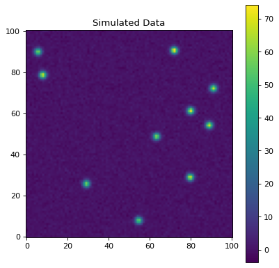
Let’s start with a simple example using simulated stars whose PSF is assumed to be Gaussian. We’ll create a synthetic image using tools provided by the photutils.datasets module:
>>> import numpy as np
>>> from photutils.datasets import make_noise_image
>>> from photutils.psf import CircularGaussianPRF, make_psf_model_image
>>> psf_model = CircularGaussianPRF(flux=1, fwhm=2.7)
>>> psf_shape = (9, 9)
>>> n_sources = 10
>>> shape = (101, 101)
>>> data, true_params = make_psf_model_image(shape, psf_model, n_sources,
...                                          model_shape=psf_shape,
...                                          flux=(500, 700),
...                                          min_separation=10, seed=0)
>>> noise = make_noise_image(data.shape, mean=0, stddev=1, seed=0)
>>> data += noise
>>> error = np.abs(noise)
Let’s plot the image:
(Source code, png, hires.png, pdf, svg)
Fitting multiple sources#
Now let’s use PSFPhotometry to perform PSF photometry
on the sources in this image. Note that the input image must be
background-subtracted prior to using the photometry classes. See
Background Estimation (photutils.background) for tools to subtract a global background from an
image. This step is not needed for our synthetic image because it does
not include background.
We’ll use the DAOStarFinder class for
source detection. We’ll estimate the initial fluxes of each
source using a circular aperture with a radius 4 pixels. The
central 5x5 pixel region of each source will be fit using an
CircularGaussianPRF PSF model. First, let’s create an
instance of the PSFPhotometry class:
>>> from photutils.detection import DAOStarFinder
>>> from photutils.psf import PSFPhotometry
>>> psf_model = CircularGaussianPRF(flux=1, fwhm=2.7)
>>> fit_shape = (5, 5)
>>> finder = DAOStarFinder(6.0, 2.0)
>>> psfphot = PSFPhotometry(psf_model, fit_shape, finder=finder,
...                         aperture_radius=4)
To perform the PSF fitting, we then call the class instance
on the data array, and optionally an error and mask array. A
NDData object holding the data, error, and mask arrays
can also be input into the data parameter. Note that all non-finite
(e.g., NaN or inf) data values are automatically masked. Here we input
the data and error arrays:
>>> phot = psfphot(data, error=error)
A table of initial PSF model parameter values can also be input when calling the class instance. An example of that is shown later.
Equivalently, one can input an NDData object with any
uncertainty object that can be converted to standard-deviation errors:
>>> from astropy.nddata import NDData, StdDevUncertainty
>>> uncertainty = StdDevUncertainty(error)
>>> nddata = NDData(data, uncertainty=uncertainty)
>>> phot2 = psfphot(nddata)
The result is an astropy Table with columns for the
source and group identification numbers, the x, y, and flux initial,
fit, and error values, local background, number of unmasked pixels
fit, the group size, quality-of-fit metrics, and flags. See the
PSFPhotometry documentation for descriptions of the
output columns.
The full table cannot be shown here as it has many columns, but let’s print the source ID along with the fit x, y, and flux values:
>>> phot['x_fit'].info.format = '.4f'  # optional format
>>> phot['y_fit'].info.format = '.4f'
>>> phot['flux_fit'].info.format = '.4f'
>>> print(phot[('id', 'x_fit', 'y_fit', 'flux_fit')])
 id  x_fit   y_fit  flux_fit
--- ------- ------- --------
  1 54.5658  7.7644 514.0091
  2 29.0865 25.6111 536.5793
  3 79.6281 28.7487 618.7642
  4 63.2340 48.6408 563.3437
  5 88.8848 54.1202 619.8904
  6 79.8763 61.1380 648.1658
  7 90.9606 72.0861 601.8593
  8  7.8038 78.5734 635.6317
  9  5.5350 89.8870 539.6831
 10 71.8414 90.5842 692.3373
Let’s create the residual image:
>>> resid = psfphot.make_residual_image(data)
and plot it:
(Source code, png, hires.png, pdf, svg)
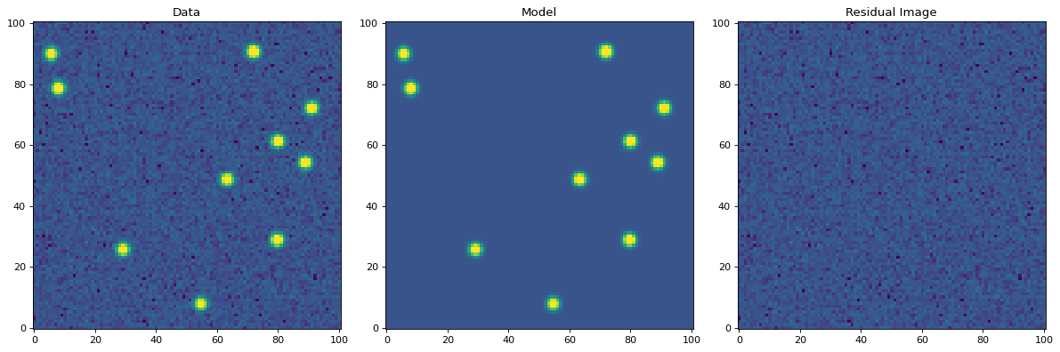
The residual image looks like noise, indicating good fits to the sources.
Further details about the PSF fitting can be obtained from attributes on
the PSFPhotometry instance. For example, the results
from the finder instance called during PSF fitting can be accessed
using the finder_results attribute (the finder returns an
astropy table):
>>> psfphot.finder_results['x_centroid'].info.format = '.4f'  # optional format
>>> psfphot.finder_results['y_centroid'].info.format = '.4f'  # optional format
>>> psfphot.finder_results['sharpness'].info.format = '.4f'  # optional format
>>> psfphot.finder_results['peak'].info.format = '.4f'
>>> psfphot.finder_results['flux'].info.format = '.4f'
>>> psfphot.finder_results['mag'].info.format = '.4f'
>>> psfphot.finder_results['daofind_mag'].info.format = '.4f'
>>> print(psfphot.finder_results)
 id x_centroid y_centroid sharpness ...   peak    flux     mag   daofind_mag
--- ---------- ---------- --------- ... ------- -------- ------- -----------
  1    54.5299     7.7460    0.6006 ... 53.5953 476.3221 -6.6948     -2.1093
  2    29.0927    25.5992    0.5955 ... 57.1982 499.4443 -6.7462     -2.1958
  3    79.6185    28.7515    0.5957 ... 65.7175 574.1382 -6.8975     -2.3401
  4    63.2485    48.6134    0.5802 ... 58.3985 521.4656 -6.7931     -2.2209
  5    88.8820    54.1311    0.5948 ... 69.1869 576.2842 -6.9016     -2.4379
  6    79.8727    61.1208    0.6216 ... 74.0935 612.8353 -6.9684     -2.4799
  7    90.9621    72.0803    0.6167 ... 68.4157 561.7163 -6.8738     -2.4035
  8     7.7962    78.5465    0.5979 ... 66.2173 595.6881 -6.9375     -2.3167
  9     5.5858    89.8664    0.5741 ... 54.3786 505.6093 -6.7595     -2.1188
 10    71.8303    90.5624    0.6038 ... 73.5747 639.9299 -7.0153     -2.4516
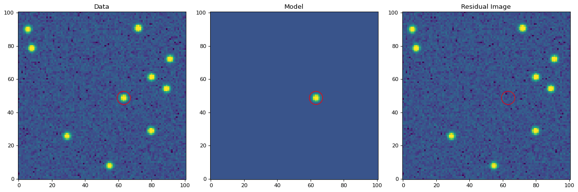
Fitting a single source#
In some cases, one may want to fit only a single source (or few sources)
in an image. We can do that by defining a table of the sources that we
want to fit. For this example, let’s fit the single source at (x,
y) = (63, 49). We first define a table with this position and then
pass that table into the init_params keyword when calling the PSF
photometry class on the data:
>>> from astropy.table import QTable
>>> init_params = QTable()
>>> init_params['x'] = [63]
>>> init_params['y'] = [49]
>>> phot = psfphot(data, error=error, init_params=init_params)
The PSF photometry class allows for flexible input column names
using a heuristic to identify the x, y, and flux columns. See
PSFPhotometry for more details.
The output table contains only the fit results for the input source:
>>> phot['x_fit'].info.format = '.4f'  # optional format
>>> phot['y_fit'].info.format = '.4f'
>>> phot['flux_fit'].info.format = '.4f'
>>> print(phot[('id', 'x_fit', 'y_fit', 'flux_fit')])
 id  x_fit   y_fit  flux_fit
--- ------- ------- --------
  1 63.2340 48.6408 563.3426
Finally, let’s show the residual image. The red circular aperture shows the location of the source that was fit and subtracted.
(Source code, png, hires.png, pdf, svg)
Forced Photometry (Fixed Model Parameters)#
In general, the three parameters fit for each source are the x and y positions and the flux. However, the astropy modeling and fitting framework allows any of these parameters to be fixed during the fitting.
Let’s say you want to fix the (x, y) position for each source. You can
do that by setting the fixed attribute on the model parameters:
>>> psf_model2 = CircularGaussianPRF(flux=1, fwhm=2.7)
>>> psf_model2.x_0.fixed = True
>>> psf_model2.y_0.fixed = True
>>> psf_model2.fixed
{'flux': False, 'x_0': True, 'y_0': True, 'fwhm': True}
Now when the model is fit, the flux will be varied but, the (x, y)
position will be fixed at its initial position for every source. Let’s
just fit a single source (defined in init_params):
>>> psfphot = PSFPhotometry(psf_model2, fit_shape, finder=finder,
...                         aperture_radius=4)
>>> phot = psfphot(data, error=error, init_params=init_params)
The output table shows that the (x, y) position was unchanged, with the fit values being identical to the initial values. However, the flux was fit:
>>> phot['flux_init'].info.format = '.4f'  # optional format
>>> phot['flux_fit'].info.format = '.4f'
>>> print(phot[('id', 'x_init', 'y_init', 'flux_init', 'x_fit',
...             'y_fit', 'flux_fit')])
 id x_init y_init flux_init x_fit y_fit flux_fit
--- ------ ------ --------- ----- ----- --------
  1     63     49  556.5067  63.0  49.0 500.2997
Bounded Model Parameters#
The astropy modeling and fitting framework also allows for bounding the parameter values during the fitting process. However, not all astropy “Fitter” classes support parameter bounds. Please see Fitting Model to Data for more details.
The model parameter bounds apply to all sources in the image,
thus this mechanism cannot be used to bound the x and y positions
of individual sources. However, the x and y positions can be
bounded for individual sources during the fitting by using the
xy_bounds keyword in PSFPhotometry and
IterativePSFPhotometry. This keyword accepts a tuple of
floats representing the maximum distance in pixels that a fitted source
can be from its initial (x, y) position.
For example, you may want to constrain the flux of a source to be
between certain values or ensure that it is a non-negative value. This
can be done by setting the bounds attribute on the input PSF model
parameters. Here we constrain the flux to be greater than or equal to
0:
>>> psf_model3 = CircularGaussianPRF(flux=1, fwhm=2.7)
>>> psf_model3.flux.bounds = (0, None)
>>> psf_model3.bounds
{'flux': (0.0, None), 'x_0': (None, None), 'y_0': (None, None), 'fwhm': (0.0, None)}
The model parameter bounds can also be set using the min and/or
max attributes. Here we set the minimum flux to be 0:
>>> psf_model3.flux.min = 0
>>> psf_model3.bounds
{'flux': (0.0, None), 'x_0': (None, None), 'y_0': (None, None), 'fwhm': (0.0, None)}
For this example, let’s constrain the flux value to be between 400 and 600:
>>> psf_model3 = CircularGaussianPRF(flux=1, fwhm=2.7)
>>> psf_model3.flux.bounds = (400, 600)
>>> psf_model3.bounds
{'flux': (400.0, 600.0), 'x_0': (None, None), 'y_0': (None, None), 'fwhm': (0.0, None)}
Source Grouping#
Source grouping is an optional feature. To turn it on, create a
SourceGrouper instance and input it via the grouper
keyword. Here we’ll group sources that are within 20 pixels of each
other:
>>> from photutils.psf import SourceGrouper
>>> grouper = SourceGrouper(min_separation=20)
>>> psfphot = PSFPhotometry(psf_model, fit_shape, finder=finder,
...                         grouper=grouper, aperture_radius=4)
>>> phot = psfphot(data, error=error)
The group_id column shows that seven groups were identified. The
sources in each group were simultaneously fit:
>>> print(phot[('id', 'group_id', 'group_size')])
 id group_id group_size
--- -------- ----------
  1        1          1
  2        2          1
  3        3          1
  4        4          1
  5        5          3
  6        5          3
  7        5          3
  8        6          2
  9        6          2
 10        7          1
Care should be taken in defining the source groups. Simultaneously
fitting very large source groups is computationally expensive and
error-prone. Internally, source grouping requires the creation of a
compound Astropy model. Due to the way compound Astropy models are
currently constructed, large groups also require excessively large
amounts of memory; this will hopefully be fixed in a future Astropy
version. A warning will be raised if the number of sources in a group
exceeds a threshold defined by the group_warning_threshold keyword.
Local Background Subtraction#
To subtract a local background from each source, define a
LocalBackground instance and input it via
the local_bkg_estimator keyword. Here we’ll use an annulus with
an inner and outer radius of 5 and 10 pixels, respectively, with the
MMMBackground statistic (with its default sigma
clipping):
>>> from photutils.background import LocalBackground, MMMBackground
>>> bkgstat = MMMBackground()
>>> local_bkg_estimator = LocalBackground(5, 10, bkg_estimator=bkgstat)
>>> finder = DAOStarFinder(10.0, 2.0)
>>> psfphot = PSFPhotometry(psf_model, fit_shape, finder=finder,
...                         grouper=grouper, aperture_radius=4,
...                         local_bkg_estimator=local_bkg_estimator)
>>> phot = psfphot(data, error=error)
The local background values are output in the table:
>>> phot['local_bkg'].info.format = '.4f'  # optional format
>>> print(phot[('id', 'local_bkg')])
 id local_bkg
--- ---------
  1   -0.0839
  2    0.1784
  3    0.2593
  4   -0.0574
  5    0.2492
  6   -0.0818
  7   -0.1130
  8   -0.2166
  9    0.0102
 10    0.3926
The local background values can also be input directly using the
init_params keyword.
Iterative PSF Photometry#
Now let’s use the IterativePSFPhotometry class to
iteratively fit the sources in the image. This class is useful for
crowded fields where faint sources are very close to bright sources. The
faint sources may not be detected until after the bright sources are
subtracted.
For this simple example, let’s input a table of three sources for the
first fit iteration. Subsequent iterations will use the finder to
find additional sources:
>>> from photutils.background import LocalBackground, MMMBackground
>>> from photutils.psf import IterativePSFPhotometry
>>> fit_shape = (5, 5)
>>> finder = DAOStarFinder(10.0, 2.0)
>>> bkgstat = MMMBackground()
>>> local_bkg_estimator = LocalBackground(5, 10, bkg_estimator=bkgstat)
>>> init_params = QTable()
>>> init_params['x'] = [54, 29, 80]
>>> init_params['y'] = [8, 26, 29]
>>> psfphot2 = IterativePSFPhotometry(psf_model, fit_shape, finder=finder,
...                                   local_bkg_estimator=local_bkg_estimator,
...                                   aperture_radius=4)
>>> phot = psfphot2(data, error=error, init_params=init_params)
The table output from IterativePSFPhotometry contains a
column called iter_detected that returns the fit iteration in which
the source was detected:
>>> phot['x_fit'].info.format = '.4f'  # optional format
>>> phot['y_fit'].info.format = '.4f'
>>> phot['flux_fit'].info.format = '.4f'
>>> print(phot[('id', 'iter_detected', 'x_fit', 'y_fit', 'flux_fit')])
 id iter_detected  x_fit   y_fit  flux_fit
--- ------------- ------- ------- --------
  1             1 54.5665  7.7641 514.2650
  2             1 29.0883 25.6092 534.0850
  3             1 79.6273 28.7480 613.0496
  4             2 63.2340 48.6415 564.1528
  5             2 88.8856 54.1203 615.4907
  6             2 79.8765 61.1359 649.9589
  7             2 90.9631 72.0880 603.7433
  8             2  7.8203 78.5821 641.8223
  9             2  5.5350 89.8870 539.5237
 10             2 71.8485 90.5830 687.4573
Estimating the FWHM of sources#
The photutils.psf package also provides a convenience function
called fit_fwhm to estimate the full width
at half maximum (FWHM) of one or more sources in an image.
This function fits the source(s) with a circular 2D Gaussian
PRF model (CircularGaussianPRF) using the
PSFPhotometry class. If your sources are not
circular or non-Gaussian, you can fit your sources using the
PSFPhotometry class using a different PSF model.
For example, let’s estimate the FWHM of the sources in our example image defined above:
>>> from photutils.psf import fit_fwhm
>>> finder = DAOStarFinder(6.0, 2.0)
>>> finder_tbl = finder(data)
>>> xypos = list(zip(finder_tbl['x_centroid'], finder_tbl['y_centroid']))
>>> fwhm = fit_fwhm(data, xypos=xypos, error=error, fit_shape=(5, 5), fwhm=2)
>>> fwhm
array([2.69735154, 2.70371211, 2.68917219, 2.69310558, 2.68931721,
       2.69804194, 2.69651045, 2.70423936, 2.71458867, 2.70285813])
Convenience Gaussian Fitting Function#
The photutils.psf package also provides a convenience function called
fit_2dgaussian() for fitting one or more sources
with a 2D Gaussian PRF model (CircularGaussianPRF)
using the PSFPhotometry class. See the function
documentation for more details and examples.