Point-like Source Detection (photutils.detection)#
Introduction#
One generally needs to identify astronomical sources in the data before
performing photometry or other measurements. The photutils.detection
subpackage provides tools to detect point-like (stellar) sources in an
image. This subpackage also provides tools to find local peaks in an
image that are above a specified threshold value.
For general-use source detection and extraction of both point-like and extended sources, please see Image Segmentation.
Detecting Stars#
Photutils includes two widely-used tools for detecting stars in an image, DAOFIND and IRAF’s starfind, plus a third tool that allows input of a custom user-defined kernel.
DAOStarFinder implements
the DAOFIND algorithm (Stetson 1987, PASP 99, 191).
It searches images for local density maxima that have a peak amplitude
above a specified threshold (applied to a convolved image) and with
size and shape similar to a defined 2D Gaussian kernel. To match the
original DAOFIND algorithm, the input threshold is internally scaled
by a factor derived from the convolution kernel. To apply the threshold
exactly as given (e.g., when supplying a spatial background-RMS map),
set scale_threshold=False. The class also computes roundness and
sharpness statistics for detected sources, with configurable lower and
upper bounds.
IRAFStarFinder is a class that
implements IRAF’s starfind algorithm. It is fundamentally
similar to DAOStarFinder, but
IRAFStarFinder always uses a circular
Gaussian kernel whereas DAOStarFinder
can use an elliptical Gaussian kernel. Another difference is that
IRAFStarFinder calculates the objects’
centroid, roundness, and sharpness using image moments.
StarFinder is a class similar to
IRAFStarFinder, but which allows input
of a custom user-defined kernel as a 2D array. This allows for more
generalization beyond simple Gaussian kernels.
The usage of IRAFStarFinder and
StarFinder follows the same pattern
as DAOStarFinder shown below. Replace
the class name and adjust the parameters (e.g., fwhm and
kernel) as needed. Note that the scale_threshold parameter
is specific to DAOStarFinder.
Note also that each class returns different output columns.
For example, DAOStarFinder
includes daofind_mag and sharpness columns, while
IRAFStarFinder includes fwhm and
pa (position angle) columns. See each class’s API documentation for
the full list of output columns.
As an example, let’s load a simulated HST star image and add Gaussian noise. We will then estimate the background and background noise using sigma-clipped statistics:
>>> import numpy as np
>>> from astropy.stats import sigma_clipped_stats
>>> from photutils.datasets import (load_simulated_hst_star_image,
...                                 make_noise_image)
>>> hdu = load_simulated_hst_star_image()
>>> data = hdu.data + make_noise_image(hdu.data.shape, distribution='gaussian', mean=10.0, stddev=5.0, seed=0)
>>> mean, median, std = sigma_clipped_stats(data, sigma=3.0)
>>> print(np.array((mean, median, std)))
[10.44410657 10.39699777  5.09141794]
Now we will subtract the background and use an instance of
DAOStarFinder to find the stars in the
image that have FWHMs of around 2.5 pixels and have peaks approximately
5 times the background standard deviation above the background (i.e.,
the threshold is 5 * std). The stars in the image are undersampled,
so we will slightly relax the sharpness_range to allow for a wider
range of values.
Running this class on the data yields an astropy QTable
containing the results of the star finder:
>>> from photutils.detection import DAOStarFinder
>>> threshold = 5.0 * std
>>> daofind = DAOStarFinder(threshold, fwhm=2.5,
...                         sharpness_range=(0.2, 1.5))
By default, DAOStarFinder internally
scales the input threshold by a factor derived from the convolution
kernel to match the original DAOFIND algorithm. To apply
the threshold exactly as given (e.g., when supplying a spatial
background-RMS map), set scale_threshold=False:
>>> daofind_unscaled = DAOStarFinder(threshold, fwhm=2.5,
...                                  sharpness_range=(0.2, 1.5),
...                                  scale_threshold=False)
Running the finder on the background-subtracted data:
>>> sources = daofind(data - median)
>>> for col in sources.colnames:
...     if col not in ('id', 'n_pixels'):
...         sources[col].info.format = '%.2f'  # for consistent table output
>>> sources.pprint(max_lines=12, max_width=76)
 id x_centroid y_centroid sharpness ...   peak    flux   mag   daofind_mag
--- ---------- ---------- --------- ... ------- ------- ------ -----------
  1     848.57       2.15      0.89 ... 1051.78 3999.02  -9.00       -3.80
  2     181.85       3.75      0.97 ... 1711.87 5568.78  -9.36       -4.28
  3     323.88       3.70      0.96 ... 3005.97 9992.14 -10.00       -4.90
  4      99.89       8.95      1.07 ... 1134.12 3236.12  -8.78       -3.77
...        ...        ...       ... ...     ...     ...    ...         ...
497     114.16     993.47      0.84 ... 1577.91 6550.22  -9.54       -4.26
498     298.44     993.87      0.83 ...  644.97 2719.64  -8.59       -3.31
499     207.21     998.15      0.97 ... 2800.62 8406.16  -9.81       -4.83
500     691.03     998.77      1.15 ... 2600.83 5612.72  -9.37       -4.64
Length = 500 rows
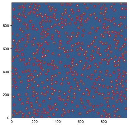
Let’s plot the image and mark the location of detected sources:
(Source code, png, hires.png, pdf, svg)
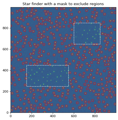
Masking Regions#
Regions of the input image can be masked by using the mask
keyword with the DAOStarFinder,
IRAFStarFinder, or
StarFinder instance. This simple example
uses DAOStarFinder and masks two
rectangular regions. No sources will be detected in the masked regions:
>>> from photutils.detection import DAOStarFinder
>>> daofind = DAOStarFinder(threshold, fwhm=2.5, sharpness_range=(0.2, 1.5))
>>> mask = np.zeros(data.shape, dtype=bool)
>>> mask[650:851, 600:851] = True
>>> mask[250:451, 150:551] = True
>>> sources = daofind(data - median, mask=mask)
(Source code, png, hires.png, pdf, svg)
Local Peak Detection#
Photutils also includes a find_peaks()
function to find local peaks in an image that are above a specified
threshold value. Peaks are the local maxima above a specified threshold
that are separated by a specified minimum number of pixels, defined by a
box size or a local footprint.
The returned pixel coordinates for the peaks are always integer-valued
(i.e., no centroiding is performed, only the peak pixel is identified).
However, a centroiding function can be input via the centroid_func
keyword to find_peaks() to also compute
centroid coordinates with subpixel precision.
The box_size parameter also effectively imposes a minimum separation
between detected peaks, since only one peak can be found within each box
of that size. Specifically, two peaks must differ by at least box_size
// 2 + 1 pixels along each axis. For example, a box_size of 11
imposes a minimum separation of 6 pixels.
As a simple example, let’s find the local peaks in the image above that are 5 sigma above the background using a box size of 11 pixels:
>>> from photutils.detection import find_peaks
>>> threshold = median + (5.0 * std)
>>> tbl = find_peaks(data, threshold, box_size=11)
>>> tbl['peak_value'].info.format = '%.8g'
>>> print(tbl)
 id x_peak y_peak peak_value
--- ------ ------ ----------
  1    849      2  1062.1752
  2    182      4  1722.2687
  3    324      4  3016.3684
  4    100      9  1144.5217
  5    824      9  1311.2049
...    ...    ...        ...
497    889    992  194.27323
498    114    994  1588.3073
499    299    994  655.36699
500    207    998  2811.0195
501    691    999  2611.2233
Length = 501 rows
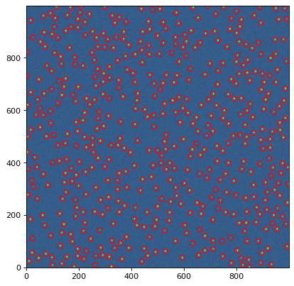
Let’s plot the location of the detected peaks in the image:
(Source code, png, hires.png, pdf, svg)