PSF Matching (photutils.psf_matching)#
Introduction#
The photutils.psf_matching subpackage contains tools to generate
kernels for matching point spread functions (PSFs). It provides two
functions for computing PSF-matching kernels in the Fourier domain:
make_kernel()— Uses the ratio of Fourier transforms with a hard amplitude threshold to regularize the division (see e.g., Gordon et al. 2008; Aniano et al. 2011).make_wiener_kernel()— Uses Wiener regularization, which smoothly suppresses noise amplification at spatial frequencies where the source response is weak.
Both functions take a source PSF and a target PSF and return a matching
kernel that, when convolved with the source PSF, produces the target
PSF. They both support an optional window function to further
suppress high-frequency noise.
How It Works#
The key idea behind both methods is that convolution in the image domain corresponds to multiplication in the Fourier domain. If the source PSF has Fourier transform \(S\) and the target PSF has Fourier transform \(T\), then the matching kernel \(K\) satisfies \(T = S \cdot K\), so \(K = T / S\).
The Fourier transform of a PSF is called the Optical Transfer Function (OTF). It describes how different spatial frequencies are transmitted through the optical system. Low frequencies (coarse image features) are typically strong in the OTF, while high frequencies (fine details) are weaker. In practice, dividing by near-zero OTF values amplifies noise. The two functions handle this differently:
make_kernel sets the Fourier ratio to zero at
frequencies where the source OTF amplitude is below a fraction of the
peak (controlled by the regularization parameter, default 1e-4):
make_wiener_kernel instead adds a
regularization term to the denominator, providing continuous, smooth
regularization. Wiener regularization smoothly down-weights frequencies
where the source response is weak, rather than zeroing them out with
a hard threshold. This typically produces matching kernels with less
ringing, especially for PSFs that have near-zero power at high spatial
frequencies.
By default, make_wiener_kernel uses a
frequency-independent scalar Tikhonov regularization term expressed as a
fraction of the peak power in the source OTF:
where \(\mathcal{F}^{-1}\) is the inverse Fourier transform,
\(S^{*}\) is the complex conjugate of \(S\), \(\lambda\) is
the regularization parameter (default 1e-4), and \(W\) is
the optional window function (defaulting to 1 if not provided).
When a penalty operator is provided (e.g., penalty='laplacian'),
the regularization becomes frequency-dependent:
where \(P\) is the OTF of the penalty operator.
A Laplacian penalty operator suppresses high spatial frequencies
more heavily, which is particularly effective at suppressing noise
amplification. Setting penalty='laplacian' reproduces the
regularization approach used by the pypher package (Boucaud et al.
2016).
For additional control, an optional window function can be applied
to both methods to further suppress high-frequency noise in the
Fourier ratios. This is especially useful for real-world PSFs that
may contain noise, diffraction artifacts, or other features that can
amplify through the division. A window is generally less critical for
make_wiener_kernel because the regularization
itself suppresses high-frequency noise. For more information about
window functions, please see Window Functions.
Choosing a Method#
Use make_kernel when:
The traditional Fourier-ratio approach with a window function is preferred (e.g., see Aniano et al. 2011).
You want fine-grained control over the spatial frequency-space filtering via a window function.
Use make_wiener_kernel when:
Working with PSFs that have near-zero power at high spatial frequencies (e.g., diffraction-limited PSFs).
You want to avoid ringing artifacts without needing to carefully tune a window function.
A single regularization parameter is preferred over choosing an OTF amplitude threshold plus a window function.
You want frequency-dependent regularization using a penalty operator (e.g.,
penalty='laplacian'forpypher-style regularization).
PSF Requirements and Preparation#
The input source and target PSFs must satisfy these requirements:
Same shape and pixel scale: Both PSFs must be 2D arrays with identical shapes and pixel scales. If your PSFs have different shapes or pixel scales, use the
resize_psf()function to resample one PSF to match the other. This function uses spline interpolation and preserves the total flux.Odd dimensions: PSF arrays should have odd dimensions in both axes to ensure a well-defined center point.
Normalized: PSF arrays should be normalized so that the sum of all pixels equals 1.
Centered (recommended but not required): The peak of the PSF should be at the center of the array.
Noiseless Gaussian Example#
For this first simple example, let’s assume our source and target PSFs are noiseless 2D Gaussians. The “high-resolution” PSF will be a Gaussian with \(\sigma=3\). The “low-resolution” PSF will be a Gaussian with \(\sigma=5\):
>>> import numpy as np
>>> from photutils.psf import CircularGaussianSigmaPRF
>>> yy, xx = np.mgrid[0:51, 0:51]
>>> gm1 = CircularGaussianSigmaPRF(flux=1, x_0=25, y_0=25, sigma=3)
>>> gm2 = CircularGaussianSigmaPRF(flux=1, x_0=25, y_0=25, sigma=5)
>>> psf1 = gm1(xx, yy)
>>> psf2 = gm2(xx, yy)
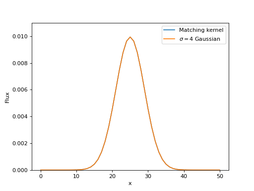
For these 2D Gaussians, the matching kernel should be a 2D Gaussian with \(\sigma=4\) (\(\sqrt{5^2 - 3^2}\)). Let’s create the matching kernel using both methods.
Using make_kernel:
>>> from photutils.psf_matching import make_kernel
>>> kernel1 = make_kernel(psf1, psf2)
Using make_wiener_kernel:
>>> from photutils.psf_matching import make_wiener_kernel
>>> kernel2 = make_wiener_kernel(psf1, psf2)
Both output kernels are 2D arrays representing the matching kernel that, when convolved with the source PSF, produces the target PSF. The output matching kernels are normalized such that they sum to 1:
>>> print(kernel1.sum())
1.0

>>> print(kernel2.sum())
1.0
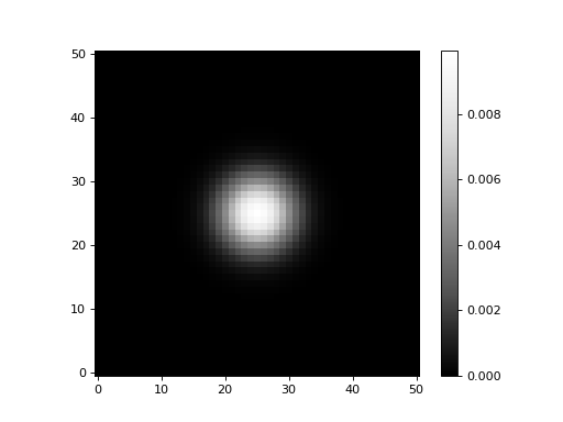
Let’s plot both results side by side:
(Source code, png, hires.png, pdf, svg)
As expected, both results are 2D Gaussians with \(\sigma=4\). Here we show 1D cuts across the center of the kernel images to confirm:
(Source code, png, hires.png, pdf, svg)
For these noiseless Gaussians, both methods produce nearly identical results. The key differences emerge when working with real-world PSFs that have significant structure in their power spectra.
Window Functions#
When working with real-world PSFs (e.g., from observations or
optical models), the Fourier ratio can still contain residual
high-frequency spatial noise even after regularization. An optional
window function
(also called a taper function) can be applied to further suppress
these artifacts. Both make_kernel() and
make_wiener_kernel() accept an optional
window parameter.
A window function multiplies the Fourier ratio by a smooth,
radially-symmetric 2D filter that equals 1.0 in the central
low-frequency region and falls to 0.0 at the edges. This filters out
high spatial frequencies where the signal-to-noise ratio is poorest.
The trade-off is that tapering removes some real information along
with the noise, so the choice of window involves balancing artifact
suppression against fidelity. A window is generally less critical for
make_wiener_kernel because the regularization
itself suppresses high-frequency noise.
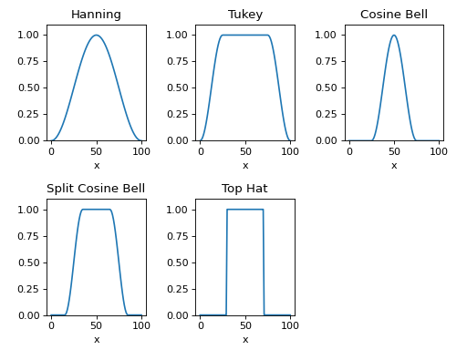
photutils.psf_matching provides five built-in window classes. They
are all subclasses of SplitCosineBellWindow,
which is parameterized by two values:
alpha: the fraction of the array radius over which the taper occurs (the cosine transition region).beta: the fraction of the array radius that remains at 1.0 (the flat inner region).
The different window classes set these parameters in specific ways, offering different levels of convenience and control.
SplitCosineBellWindow#
The split cosine bell is the most general window, taking both alpha
and beta as independent parameters. The window equals 1.0 for
radii less than beta times the maximum radius, tapers over the
next alpha fraction, and is zero beyond. Use this when you need
fine-grained control over both the preserved region and the taper width.
TukeyWindow#
The Tukey window (beta
= 1 - alpha) features a flat central plateau at 1.0 surrounded by a
cosine taper. The alpha parameter controls the fraction of the array
that is tapered: smaller alpha preserves more data but provides less
artifact suppression, while larger alpha tapers more aggressively.
When alpha=0 it becomes a TopHatWindow;
when alpha=1 it becomes a HanningWindow.
This window provides a good balance and is a solid general-purpose
choice.
HanningWindow#
The Hann window
(alpha=1.0, beta=0.0) is a raised cosine that equals 1.0 only at
the exact center and smoothly tapers to zero at the edges. The entire
array is tapered. This provides the strongest sidelobe suppression in
Fourier space, at the cost of attenuating most of the data. Use this
when edge artifacts and ringing are a primary concern.
CosineBellWindow#
The cosine bell window (alpha=alpha, beta=0.0) equals 1.0 at
the center and begins tapering immediately outward using a cosine
function over a fraction alpha of the array radius. Beyond
the taper region the window is zero. When alpha=1, this is
equivalent to a HanningWindow. Compared to
a TukeyWindow with the same alpha, the
cosine bell has no flat plateau, so the taper starts closer to the
center.
TopHatWindow#
The top hat window (alpha=0.0, beta=beta) equals 1.0 inside
a circular region and drops sharply to 0.0 outside with no smooth
transition. This preserves all data within the cutoff radius but the
sharp edge creates strong ringing artifacts in Fourier space. For most
PSF matching applications, TukeyWindow is
generally preferred over this window.
Custom Window Functions#
Users may also define their own custom window function and
pass it to make_kernel() or
make_wiener_kernel(). The window function
should be a callable that takes a single shape argument (a tuple
defining the 2D array shape) and returns a 2D array of the same shape
containing the window values. The window values should range from 0.0
to 1.0, where 1.0 indicates full preservation of that spatial frequency
and 0.0 indicates complete suppression. The window should be radially
symmetric and centered on the array.
Example Window Function Plots#
Here are plots of 1D cuts across the center of each 2D window function defined above:
(Source code, png, hires.png, pdf, svg)
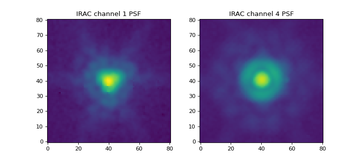
Matching Spitzer IRAC PSFs#
For this example, let’s generate a matching kernel to go
from the Spitzer/IRAC channel 1 (3.6 microns) PSF to the
channel 4 (8.0 microns) PSF. We load the PSFs using the
load_irac_psf() convenience function:
>>> from photutils.datasets import load_irac_psf
>>> ch1_hdu = load_irac_psf(channel=1)
>>> ch4_hdu = load_irac_psf(channel=4)
>>> ch1_psf = ch1_hdu.data
>>> ch4_psf = ch4_hdu.data
Let’s display the images:
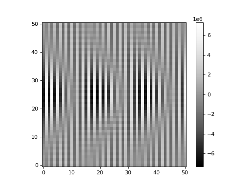
(Source code, png, hires.png, pdf, svg)
Note that these Spitzer/IRAC channel 1 and 4 PSFs have the same
shape and pixel scale. If that is not the case, one can use the
resize_psf() convenience function
to resize a PSF image. Typically, one would interpolate the
lower-resolution PSF to the same size as the higher-resolution PSF.
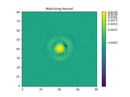
For real-world PSFs like these, applying a window function is
recommended for make_kernel() to
suppress residual high-frequency artifacts. Here we use the
SplitCosineBellWindow:
>>> from photutils.psf_matching import (SplitCosineBellWindow,
...                                     make_kernel)
>>> window = SplitCosineBellWindow(alpha=0.15, beta=0.3)
>>> kernel1 = make_kernel(ch1_psf, ch4_psf, window=window,
...                       regularization=0.0001)
With make_wiener_kernel(), the Wiener
regularization itself suppresses high-frequency noise, so a window
function is generally not needed:
>>> from photutils.psf_matching import make_wiener_kernel
>>> kernel2 = make_wiener_kernel(ch1_psf, ch4_psf,
...                              regularization=0.0001)
For frequency-dependent regularization using a Laplacian or biharmonic penalty operator:
>>> kernel3 = make_wiener_kernel(ch1_psf, ch4_psf,
...                              regularization=0.0001,
...                              penalty='laplacian')
>>> kernel4 = make_wiener_kernel(ch1_psf, ch4_psf,
...                              regularization=0.0001,
...                              penalty='biharmonic')
Let’s display the matching kernel results from all methods:
(Source code, png, hires.png, pdf, svg)
Let’s now convolve the channel 1 PSF with each matching kernel using
scipy.signal.fftconvolve and compare the PSF-matched results with the
channel 4 PSF:
(Source code, png, hires.png, pdf, svg)
Now let’s examine the residuals between the PSF-matched results and the channel 4 PSF target:
(Source code, png, hires.png, pdf, svg)

The residuals are small relative to the peak PSF values, confirming that all four methods produce good PSF matches.
Finally, let’s compare the encircled energies of the PSF-matched
results with the channel 1 and channel 4 PSFs using the
CurveOfGrowth class. A residual subpanel
immediately below the main panel shows how well each PSF-matched curve
agrees with the channel 4 target:
(Source code, png, hires.png, pdf, svg)

The encircled energy curves for the PSF-matched results closely track the channel 4 PSF, confirming that the PSF matching has been performed successfully across all four methods. The residual subpanel quantifies the small remaining differences between each PSF-matched curve and the channel 4 target.