
Building an effective Point Spread Function (ePSF)#
The ePSF#
The instrumental PSF is a combination of many factors that are generally difficult to model. Anderson and King 2000 (PASP 112, 1360) showed that accurate stellar photometry and astrometry can be derived by modeling the net PSF, which they call the effective PSF (ePSF). The ePSF is an empirical model describing what fraction of a star’s light will land in a particular pixel. The constructed ePSF is typically oversampled with respect to the detector pixels.
The oversampling in the ePSF is crucial because it captures the PSF pixel phase effect. Since stars can land at fractional pixel positions on the detector, the PSF appearance varies depending on the star’s position within a pixel. By building an oversampled ePSF, we capture this phase information across the full pixel-to-pixel variation. This allows for more accurate PSF modeling and improved photometric measurements, as the PSF can be interpolated to the exact position of any star.
Building an ePSF#
Photutils provides tools for building an ePSF following the prescription of Anderson and King 2000 (PASP 112, 1360) and subsequent enhancements detailed mainly in Anderson 2016 (WFC3 ISR 2016-12). The process iteratively refines the ePSF model and star positions: the current ePSF is fitted to the stars to improve their centers, and then the ePSF is rebuilt using the improved star positions.
To begin, we must first define a sample of stars used to build the
ePSF. Ideally these stars should be bright (high S/N) and isolated to
prevent contamination from nearby stars. One may use the star-finding
tools in Photutils (e.g., DAOStarFinder
or IRAFStarFinder) to identify an initial
sample of stars. However, the step of creating a good sample of stars
generally requires visual inspection and manual selection to ensure
stars are sufficiently isolated and of good quality (e.g., no cosmic
rays, detector artifacts, etc.). To produce a good ePSF, one should have
a reasonably large sample of stars (e.g., several hundred) in order to
fully sample the PSF over the oversampled grid and to help reduce the
effects of noise. Otherwise, the resulting ePSF may have holes or may be
noisy.
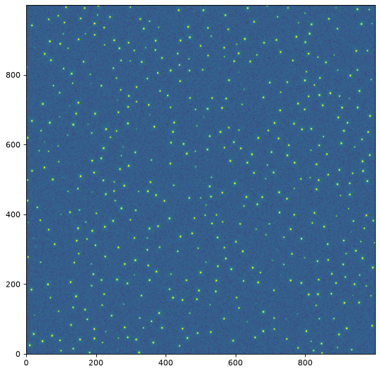
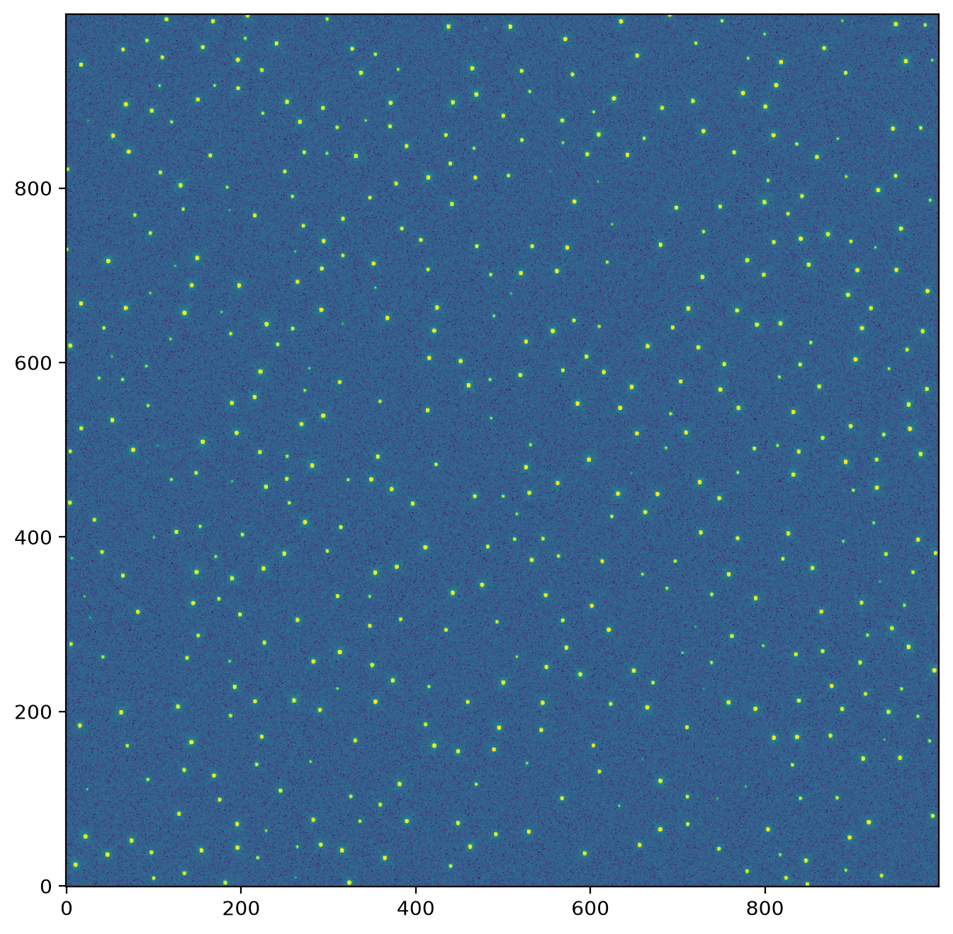
Let’s start by loading a simulated HST/WFC3 image in the F160W band:
>>> from photutils.datasets import load_simulated_hst_star_image
>>> hdu = load_simulated_hst_star_image()
>>> data = hdu.data
The simulated image does not contain any background or noise, so let’s add those to the image:
>>> from photutils.datasets import make_noise_image
>>> data += make_noise_image(data.shape, distribution='gaussian',
...                          mean=10.0, stddev=5.0, seed=0)
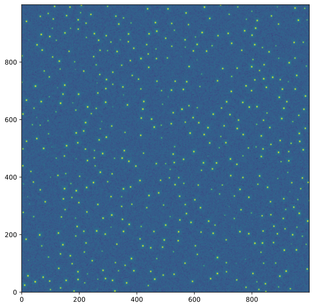
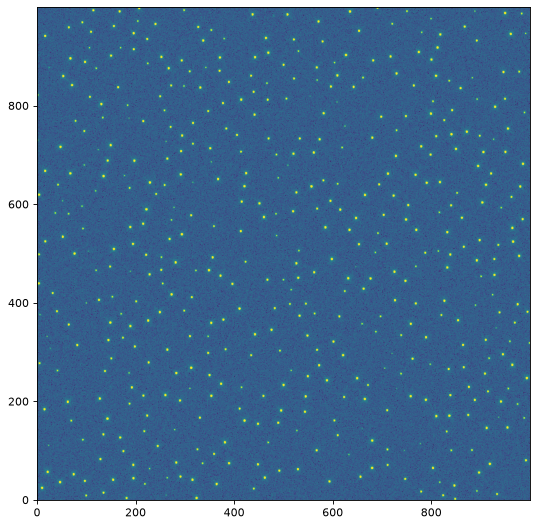
Let’s show the image:
import matplotlib.pyplot as plt
from astropy.visualization import simple_norm
from photutils.datasets import (load_simulated_hst_star_image,
                                make_noise_image)

hdu = load_simulated_hst_star_image()
data = hdu.data
data += make_noise_image(data.shape, distribution='gaussian', mean=10.0,
                         stddev=5.0, seed=0)

fig, ax = plt.subplots(figsize=(8, 8))
norm = simple_norm(data, 'sqrt', percent=99.0)
ax.imshow(data, norm=norm, origin='lower')
(Source code, png, hires.png, pdf, svg)
For this example we’ll use the
DAOStarFinder class to identify the
brighter stars and their initial positions:
>>> from photutils.detection import DAOStarFinder
>>> finder = DAOStarFinder(threshold=100.0, fwhm=1.5)
>>> sources = finder(data)
>>> for col in sources.colnames:
...     if col not in ('id', 'n_pixels'):
...         sources[col].info.format = '%.2f'  # for consistent table output
>>> sources.pprint(max_width=76)
 id x_centroid y_centroid sharpness ...   peak    flux    mag   daofind_mag
--- ---------- ---------- --------- ... ------- -------- ------ -----------
  1     848.53       2.15      0.87 ... 1062.18  4258.95  -9.07       -2.41
  2     181.85       3.74      0.91 ... 1722.27  5828.71  -9.41       -2.93
  3     323.87       3.69      0.91 ... 3016.37 10252.06 -10.03       -3.55
  4      99.89       8.95      0.96 ... 1144.52  3496.04  -8.86       -2.47
  5     824.12       9.36      0.90 ... 1311.20  4685.32  -9.18       -2.64
...        ...        ...       ... ...     ...      ...    ...         ...
478     888.44     991.86      0.85 ...  194.27  1005.88  -7.51       -0.52
479     114.16     993.40      0.84 ... 1588.31  6810.15  -9.58       -2.84
480     298.36     993.87      0.84 ...  655.37  2979.57  -8.69       -1.88
481     207.21     998.17      0.91 ... 2811.02  8614.10  -9.84       -3.48
482     691.02     998.77      0.98 ... 2611.22  5768.68  -9.40       -3.39
Length = 482 rows
Let’s show the detected stars overlaid on the image:
(Source code, png, hires.png, pdf, svg)
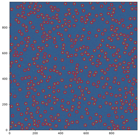
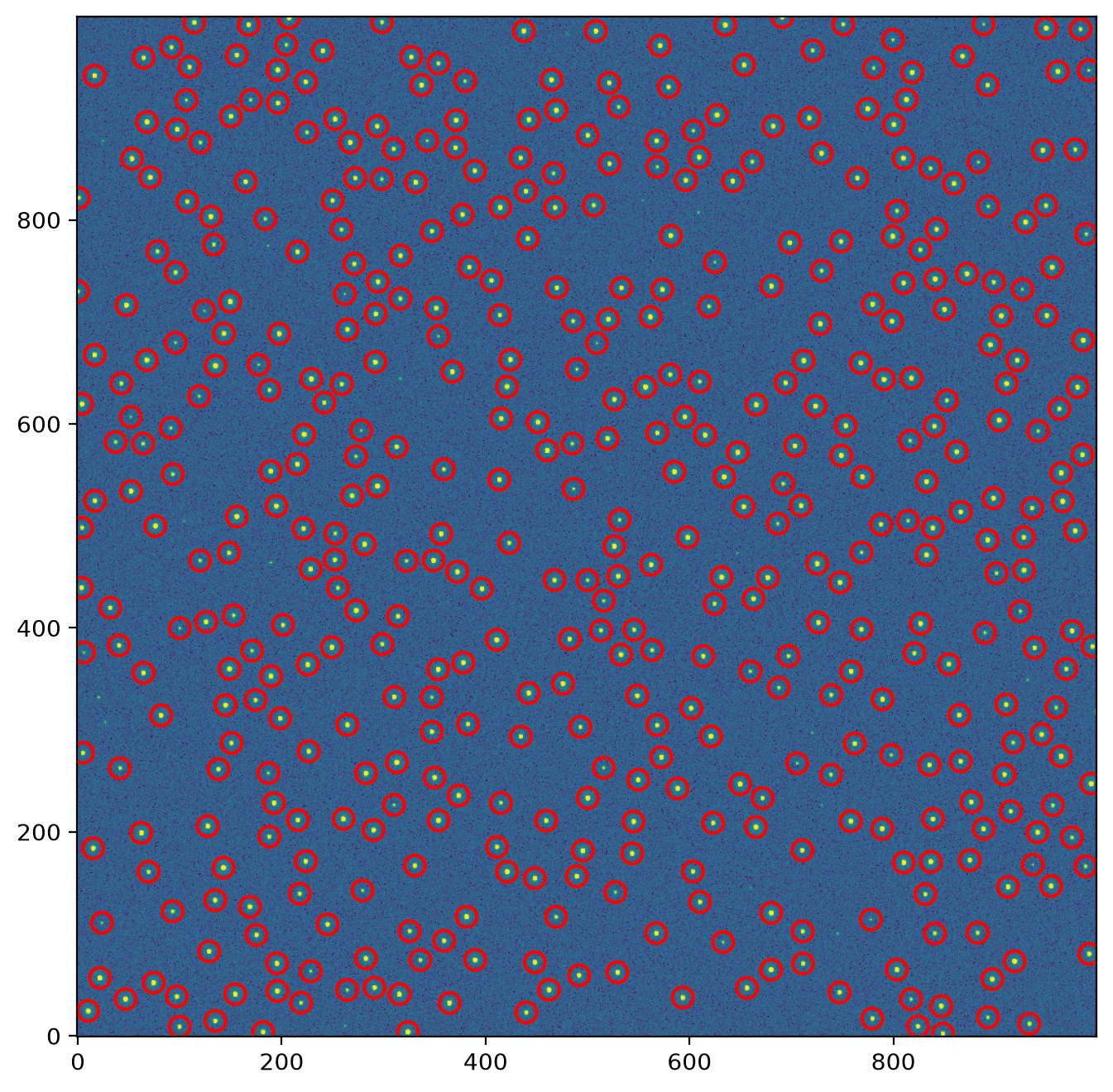
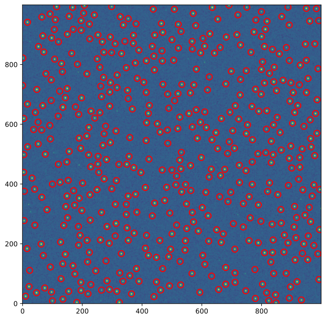
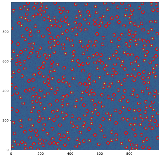
Note that the stars are sufficiently separated in the simulated image that we do not need to exclude any stars due to crowding. In practice this step will require some manual inspection and selection.
Extracting Star Cutouts#
Next, we need to extract cutouts of the stars using the
extract_stars() function. This function requires
a table of star positions either in pixel or sky coordinates. For this
example we are using pixel coordinates, which need to be in table
columns called x and y.
We’ll extract 25 x 25 pixel cutouts of our selected stars. Let’s explicitly exclude stars that are too close to the image boundaries (because they cannot be extracted):
>>> size = 25
>>> hsize = (size - 1) / 2
>>> x = sources['x_centroid']
>>> y = sources['y_centroid']
>>> mask = ((x > hsize) & (x < (data.shape[1] - 1 - hsize)) &
...         (y > hsize) & (y < (data.shape[0] - 1 - hsize)))
Now let’s create the table of good star positions:
>>> from astropy.table import Table
>>> stars_tbl = Table()
>>> stars_tbl['x'] = x[mask]
>>> stars_tbl['y'] = y[mask]
The star cutouts from which we build the ePSF must have the
background subtracted. Here we’ll use the sigma-clipped median value
as the background level. If the background in the image varies
across the image, one should use more sophisticated methods (e.g.,
Background2D).
Let’s subtract the background from the image:
>>> from astropy.stats import sigma_clipped_stats
>>> mean_val, median_val, std_val = sigma_clipped_stats(data, sigma=2.0)
>>> data -= median_val
The extract_stars() function requires the input
data as an NDData object. An NDData
object is easy to create from our data array:
>>> from astropy.nddata import NDData
>>> nddata = NDData(data=data)
We are now ready to create our star cutouts using the
extract_stars() function. For this simple example
we are extracting stars from a single image using a single catalog. The
extract_stars() function can also extract stars
from multiple images using a separate catalog for each image or a single
catalog. When using a single catalog with multiple images, the star
positions must be in sky coordinates (as SkyCoord
objects) and the NDData objects must contain valid
WCS objects. In the case of using multiple images (i.e.,
dithered images) and a single catalog, the same physical star will be
“linked” across images, meaning it will be constrained to have the same
sky coordinate in each input image.
Let’s extract the 25 x 25 pixel cutouts of our selected stars:
>>> from photutils.psf import extract_stars
>>> stars = extract_stars(nddata, stars_tbl, size=25)
The function returns an EPSFStars object containing the
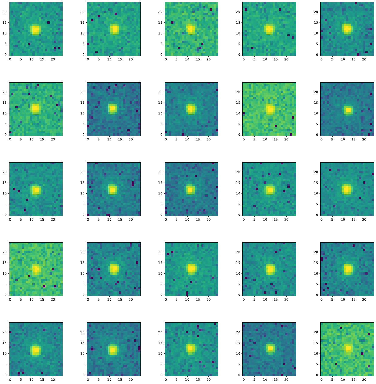
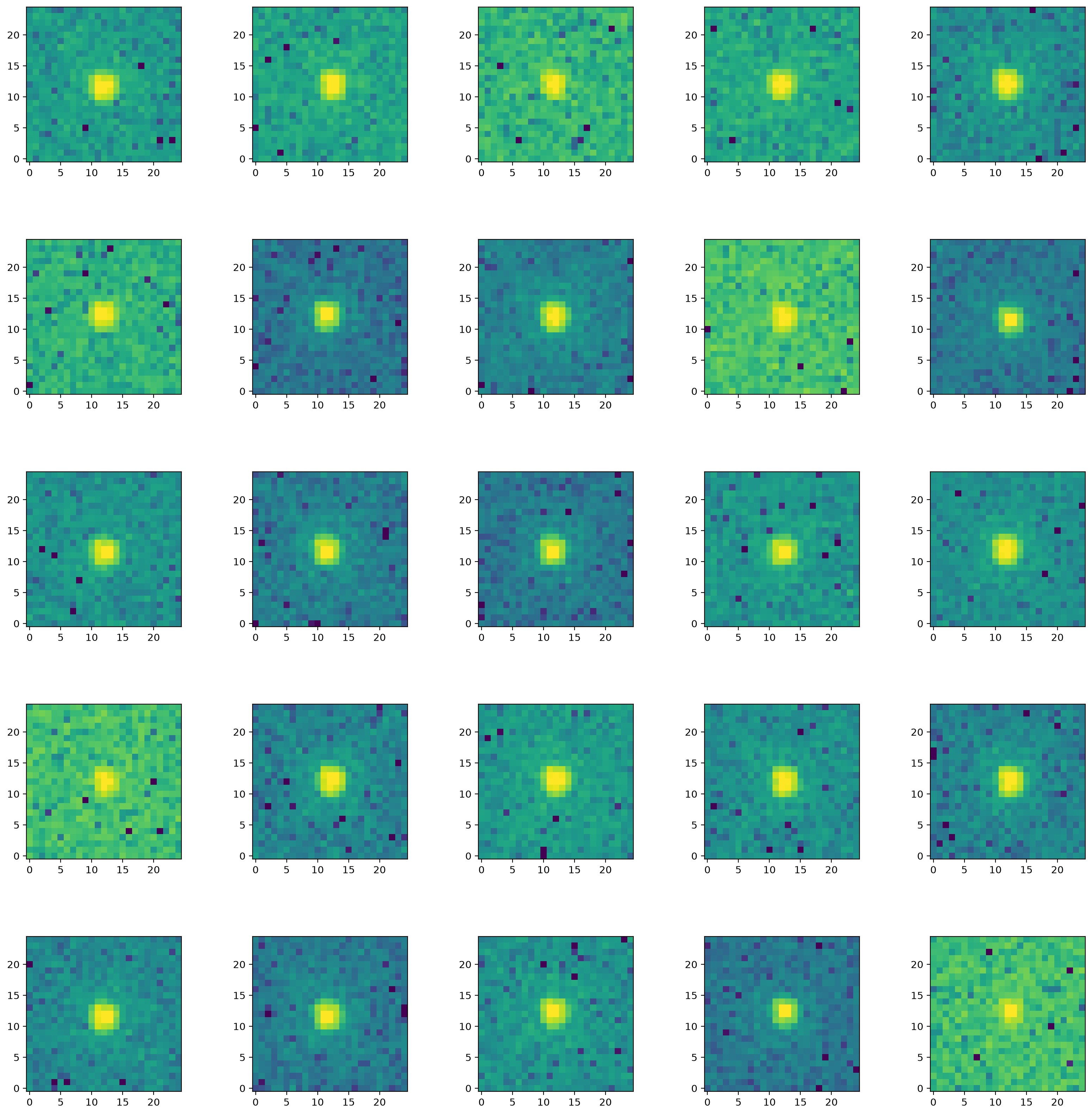
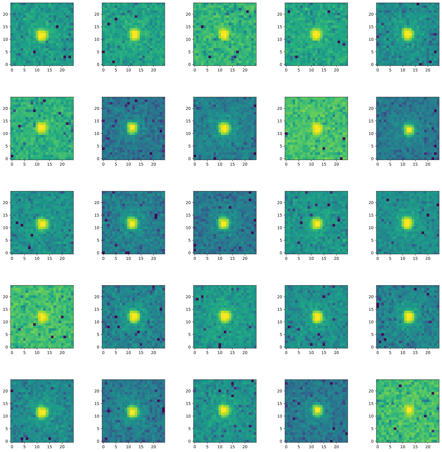
cutouts of our selected stars that will be used to build the ePSF. Let’s
show the first 25 of them:
>>> import matplotlib.pyplot as plt
>>> from astropy.visualization import simple_norm
>>> nrows = 5
>>> ncols = 5
>>> fig, ax = plt.subplots(nrows=nrows, ncols=ncols, figsize=(20, 20),
...                        squeeze=True)
>>> ax = ax.ravel()
>>> for i in range(nrows * ncols):
...     norm = simple_norm(stars[i], 'log', percent=99.0)
...     ax[i].imshow(stars[i], norm=norm, origin='lower')
(Source code, png, hires.png, pdf, svg)

Constructing the ePSF#
With the star cutouts, we are ready to construct the ePSF with the
EPSFBuilder class. We’ll create an ePSF with
an oversampling factor of 4. Here we limit the maximum number of
iterations to 3 (to limit its run time), but in practice one should use
about 10 or more iterations. The EPSFBuilder
class has many options to control the ePSF build process, including
changing the recentering function, the smoothing kernel, and the
convergence accuracy. Please see the EPSFBuilder
documentation for further details.
We first initialize an EPSFBuilder instance with
our desired parameters and then input the cutouts of our selected stars
to the instance:
>>> from photutils.psf import EPSFBuilder
>>> epsf_builder = EPSFBuilder(oversampling=4, maxiters=3,
...                            progress_bar=False)
>>> result = epsf_builder(stars)
The EPSFBuilder returns an
EPSFBuildResults object containing the constructed ePSF,
the fitted stars, and detailed information about the build process. This
result object supports tuple unpacking, so both of the following work:
>>> # New style: access result attributes
>>> epsf = result.epsf
>>> fitted_stars = result.fitted_stars

>>> # Old style: tuple unpacking still works
>>> epsf, fitted_stars = epsf_builder(stars)
The EPSFBuildResults object provides useful diagnostic
information about the build process:
>>> result.converged
np.False_
>>> result.iterations
3
>>> result.n_excluded_stars
0
The returned epsf is an ImagePSF object, and
fitted_stars is a new EPSFStars object with the
updated star positions and fluxes from fitting the final ePSF model.
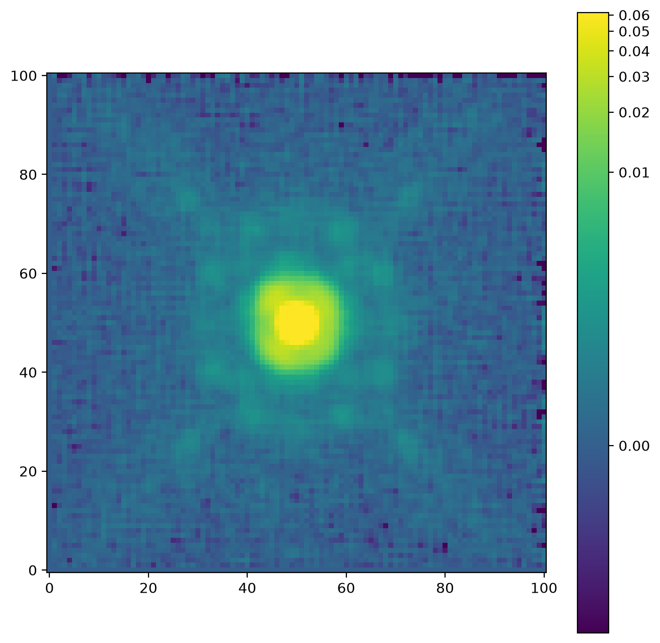
Finally, let’s show the constructed ePSF:
>>> import matplotlib.pyplot as plt
>>> from astropy.visualization import simple_norm
>>> fig, ax = plt.subplots(figsize=(8, 8))
>>> norm = simple_norm(epsf.data, 'log', percent=99.0)
>>> axim = ax.imshow(epsf.data, norm=norm, origin='lower')
>>> fig.colorbar(axim)
(Source code, png, hires.png, pdf, svg)
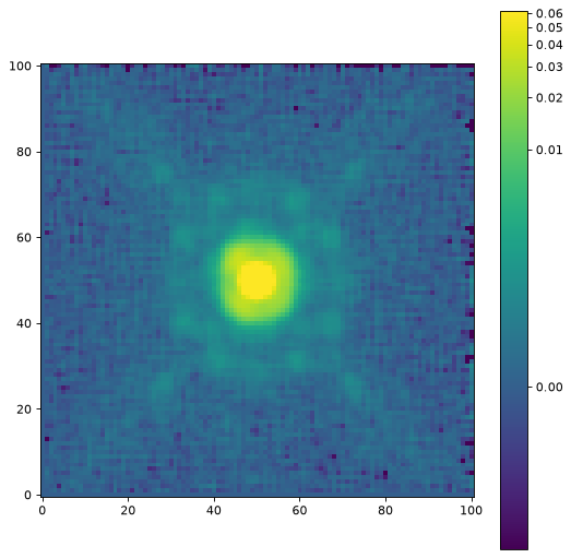
The ImagePSF object can be
used as a PSF model for PSF Photometry (i.e., PSFPhotometry or
IterativePSFPhotometry).
Customizing the ePSF Builder#
The EPSFBuilder class provides several options
to customize the ePSF build process.
Smoothing Kernel#
The smoothing_kernel parameter controls the smoothing applied to
the ePSF during each iteration. The smoothing helps to reduce noise in
the ePSF, especially when the number of stars is small. The default
is 'quartic', which uses a fourth-degree polynomial kernel. This
kernel was initially developed by Anderson and King for HST data with an
ePSF oversampling factor of 4. It is designed to provide a good balance
between smoothing and preserving the shape of the ePSF.
You can also use 'quadratic' for a second-degree polynomial kernel,
provide a custom 2D array, or set it to None for no smoothing:
>>> epsf_builder = EPSFBuilder(oversampling=4, maxiters=3,
...                            smoothing_kernel='quadratic',
...                            progress_bar=False)
Customizing the ePSF Fitting#
The EPSFBuilder class allows you to customize
the fitting process using the fit_shape parameter. This parameter
specifies the size of the box (in pixels) centered on each star used
for fitting. Using a smaller box can speed up the fitting process while
still capturing the core of the PSF:
>>> epsf_builder = EPSFBuilder(oversampling=4, maxiters=3,
...                            fit_shape=7,
...                            progress_bar=False)
You can also customize the fitter itself by passing a
Fitter instance:
>>> from astropy.modeling.fitting import LMLSQFitter
>>> fitter = LMLSQFitter()
>>> epsf_builder = EPSFBuilder(oversampling=4, maxiters=3,
...                            fitter=fitter, fit_shape=7,
...                            progress_bar=False)
Sigma Clipping#
The sigma_clip parameter controls the sigma clipping applied when
stacking the ePSF residuals in each iteration. The default uses sigma
clipping with sigma=3.0 and maxiters=10. You can provide your
own SigmaClip instance to customize this behavior:
>>> from astropy.stats import SigmaClip
>>> sigclip = SigmaClip(sigma=2.5, maxiters=5)
>>> epsf_builder = EPSFBuilder(oversampling=4, maxiters=3,
...                            sigma_clip=sigclip,
...                            progress_bar=False)
Including Weights#
If your input NDData object contains uncertainty
information, the extract_stars() function will
automatically create weights for each star cutout. These weights are
used during the ePSF fitting process to give more weight to pixels with
lower uncertainties.
To include weights, provide an uncertainty attribute in
your NDData object. The uncertainty can be
any of the NDUncertainty subclasses (e.g.,
StdDevUncertainty):
>>> from astropy.nddata import StdDevUncertainty
>>> uncertainty = StdDevUncertainty(np.sqrt(np.abs(data)))
>>> nddata = NDData(data=data, uncertainty=uncertainty)
Linked Stars for Dithered Images#
When building an ePSF from multiple dithered images, you can link
stars across images to ensure they are constrained to have the same
sky coordinates. This is done by providing a single catalog with sky
coordinates and multiple NDData objects, each with a
valid WCS.
The extract_stars() function will create
LinkedEPSFStar objects that link the corresponding star
cutouts from each image. During the ePSF building process, linked stars
are constrained to have the same sky coordinate across all images.
>>> from astropy.coordinates import SkyCoord
>>> catalog = Table()
>>> catalog['skycoord'] = SkyCoord(ra=[...]*u.deg, dec=[...]*u.deg)
>>> stars = extract_stars([nddata1, nddata2], catalog, size=25)