Aperture Photometry (`photutils.aperture`)#

Introduction#

The AperturePhotometry class and the ApertureStats class are the primary tools for performing aperture photometry. They work in conjunction with the aperture classes.

The AperturePhotometry class sums the (weighted) data values within one or more apertures and reports the aperture fluxes, uncertainties, unmasked overlap areas, and bitwise quality flags. The ApertureStats class computes per-source statistics (e.g., mean, median, standard deviation, sigma-clipped values, and morphological properties) for the pixels within an aperture. The legacy aperture_photometry() function performs basic aperture photometry, returning only the aperture sums and (optionally) their uncertainties. It is retained for backwards compatibility, but new features are added only to the AperturePhotometry and ApertureStats classes.

Tip

Which tool should I use?

Use AperturePhotometry for aperture fluxes (sums), errors, areas and quality flags. The calculated values can be accessed as class attributes or output as an Astropy QTable. For aperture photometry, it is faster than ApertureStats.
Use ApertureStats for per-source statistics such as the median, standard deviation, sigma-clipped values, and morphological properties.
Use the legacy aperture_photometry() function only if you need its original output columns for backwards compatibility.

Apertures#

Photutils provides several apertures defined in pixel or sky coordinates.

Pixel coordinates	Sky coordinates
`CircularAperture`	`SkyCircularAperture`
`CircularAnnulus`	`SkyCircularAnnulus`
`EllipticalAperture`	`SkyEllipticalAperture`
`EllipticalAnnulus`	`SkyEllipticalAnnulus`
`RectangularAperture`	`SkyRectangularAperture`
`RectangularAnnulus`	`SkyRectangularAnnulus`
`PolygonAperture`	`SkyPolygonAperture`

The AperturePhotometry class and the ApertureStats class both accept Aperture objects. When using sky-based apertures, a WCS transformation must also be provided.

They also accept supported regions.Region objects, i.e., region classes that correspond to the aperture classes listed above. The AperturePhotometry class additionally accepts a list of Aperture and/or regions.Region objects, provided they all have identical positions.

The region_to_aperture() convenience function can be used to convert a regions.Region object to the corresponding Aperture object.

Creating Aperture Objects#

The first step in performing aperture photometry is to create an aperture object. An aperture is defined by one or more positions and the parameters that specify its size and, where applicable, its orientation (e.g., for elliptical apertures).

The following example creates a circular aperture in pixel coordinates using the CircularAperture class:

>>> from photutils.aperture import CircularAperture
>>> positions = [(71.4, 23.9), (42.1, 41.7), (54.6, 68.2)]
>>> aperture = CircularAperture(positions, r=3.1)

The positions can be specified as a single (x, y) tuple, a list of (x, y) tuples, or an N×2 array, where N is the number of positions. In this example, three circular apertures with a radius of 3.1 pixels are created at (x, y) pixel coordinates (71.4, 23.9), (42.1, 41.7), and (54.6, 68.2).

Creating an aperture in sky coordinates is similar. First, define the sky coordinates using the SkyCoord class, then create the aperture using the SkyCircularAperture class:

>>> from astropy import units as u
>>> from astropy.coordinates import SkyCoord
>>> from photutils.aperture import SkyCircularAperture
>>> positions = SkyCoord([101.20, 101.21], [45.14, 45.12], unit='deg',
...                      frame='icrs')
>>> aperture = SkyCircularAperture(positions, r=4.0 * u.arcsec)

Note

Sky apertures are not defined entirely in sky coordinates. The aperture center is specified by sky coordinates, while the aperture size is specified in angular units, and the orientation (theta, where applicable) is defined in the sky coordinate frame. When converting to pixel coordinates, the aperture size and orientation are transformed using the local pixel scale and rotation at the aperture center. Projection distortions are not taken into account.

Consequently, sky apertures are not apertures defined on the celestial sphere. Instead, they represent aperture shapes on an image that are anchored to a sky position. This design preserves the aperture shape when converting between sky and pixel coordinates, which would not generally be possible if the aperture were defined as a true region on the celestial sphere.

Converting Between Pixel and Sky Apertures#

The pixel apertures can be converted to sky apertures, and vice versa, given a WCS object. To convert a pixel aperture to a sky aperture, use the to_sky() method. The following example shows how to convert a CircularAperture to a SkyCircularAperture using a sample WCS object:

>>> from photutils.datasets import make_wcs
>>> wcs = make_wcs((100, 100))
>>> aperture = CircularAperture((12.3, 18.7), r=4.0)
>>> sky_aperture = aperture.to_sky(wcs)
>>> sky_aperture
<SkyCircularAperture(<SkyCoord (ICRS): (ra, dec) in deg
    (197.89228076, -1.36685926)>, r=0.39999999972155825 arcsec)>

To convert a sky aperture to a pixel aperture, use the to_pixel() method:

>>> position = SkyCoord(197.89228076, -1.36685926, unit='deg',
...                     frame='icrs')
>>> aperture = SkyCircularAperture(position, r=0.4 * u.arcsec)
>>> pix_aperture = aperture.to_pixel(wcs)
>>> pix_aperture
<CircularAperture([12.29985329, 18.700118  ], r=4.000000002260265)>

By default, a circular aperture converts to a circle whose radius is scaled by the mean pixel scale. A circle on the sky maps to an ellipse in pixel coordinates (and vice versa) whenever the pixels are not square or the WCS is sheared. Pass as_ellipse=True to the to_pixel or to_sky method of a circular aperture or annulus to return that ellipse instead. For example, with pixels that are 0.1 arcsec wide and 0.2 arcsec tall, a 0.4 arcsec sky circle becomes a pixel ellipse with semi-axes of 4 and 2 pixels:

>>> from astropy.wcs import WCS
>>> wcs2 = WCS(naxis=2)
>>> wcs2.wcs.ctype = ['RA---TAN', 'DEC--TAN']
>>> wcs2.wcs.crval = [197.89228076, -1.36685926]
>>> wcs2.wcs.crpix = [50.0, 50.0]
>>> wcs2.wcs.cdelt = [-0.1 / 3600, 0.2 / 3600]
>>> ellipse = aperture.to_pixel(wcs2, as_ellipse=True)
>>> print(ellipse.a, ellipse.b)
3.999999998537498 2.0000000002783653

Note

Each aperture has a single fixed shape that is applied identically at every position (e.g., a circular pixel aperture has the same radius at all positions). However, a WCS may have a spatially varying pixel scale, rotation, or distortion, so there is generally no single transformation that preserves the aperture shape at every position simultaneously.

To ensure a deterministic conversion, the local WCS properties (e.g., pixel scale and rotation angle) are computed at a single reference position. By convention, this is the first aperture position. This behavior applies to all aperture classes, including PolygonAperture and SkyPolygonAperture, whose vertex offsets are transformed using the WCS evaluated at the first position.

Consequently, when converting apertures with multiple positions using a WCS with significant spatial variations, the converted aperture shapes may become increasingly inaccurate for positions farther from the first position.

Polygon Apertures#

In addition to the built-in circular, elliptical, and rectangular shapes, arbitrary polygon apertures are supported via the PolygonAperture and SkyPolygonAperture classes. Like the other aperture types, a polygon aperture has a single fixed shape (defined by its vertex_offsets) that can be applied at one or more positions:

>>> import numpy as np
>>> from photutils.aperture import PolygonAperture
>>> positions = [(71.4, 23.9), (42.1, 41.7), (54.6, 68.2)]
>>> offsets = [(-3.0, -2.0), (3.0, -2.0), (3.0, 2.0), (-3.0, 2.0)]
>>> aperture = PolygonAperture(positions, offsets)

The polygon must be simple (non-self-intersecting) with at least three vertices, but it does not need to be convex. Non-convex shapes such as L-shapes or stars are fully supported. The vertices may be input in either clockwise or counter-clockwise order. They are normalized to counter-clockwise order internally.

A single polygon can also be constructed directly from its absolute vertex coordinates using the from_vertices() class method, which sets the aperture position to the polygon centroid:

>>> vertices = [(0.0, 0.0), (4.0, 0.0), (4.0, 3.0)]
>>> aperture = PolygonAperture.from_vertices(vertices)

Regular polygons (equal-length sides and equal interior angles) can be created with the from_regular_polygon() class method by specifying a center, the number of vertices, the outer radius (circumradius), and an optional rotation angle:

>>> hexagon = PolygonAperture.from_regular_polygon((31.4, 32.9),
...                                                n_vertices=6,
...                                                radius=5.0)

For regular polygons, the outer_radius, inner_radius, side_length, interior_angle, exterior_angle, and theta properties expose the geometric parameters of the shape.

Converting to Polygon Apertures#

The built-in CircularAperture, EllipticalAperture, RectangularAperture, SkyCircularAperture, SkyEllipticalAperture, and SkyRectangularAperture classes provide a to_polygon method that returns a PolygonAperture or SkyPolygonAperture. For circular and elliptical apertures, the returned polygon approximates the aperture boundary. For rectangular apertures, it is exactly equivalent.

Performing Aperture Photometry#

After the aperture object is created, we can then perform the photometry using the AperturePhotometry class. We start by defining the aperture (at three positions) as described above:

>>> from photutils.aperture import CircularAperture
>>> positions = [(71.4, 23.9), (42.1, 41.7), (54.6, 68.2)]
>>> aperture = CircularAperture(positions, r=3.1)

We then create an AperturePhotometry instance with the data and the apertures. Note that AperturePhotometry assumes that the input data have been background subtracted. For simplicity, we define the data here as an array of all ones:

>>> import numpy as np
>>> from photutils.aperture import AperturePhotometry
>>> data = np.ones((100, 100))
>>> phot = AperturePhotometry(data, aperture)

The aperture fluxes, uncertainties, unmasked overlap areas, and quality flags are available as lazily-computed attributes (see flux, flux_err, area, and flags):

>>> print(phot.flux)
[30.1907054 30.1907054 30.1907054]

The results can also be output as an Astropy QTable using the to_table() method:

>>> phot_table = phot.to_table()
>>> phot_table['flux'].info.format = '%.8g'  # for consistent table output
>>> phot_table['area'].info.format = '%.8g'  # for consistent table output
>>> phot_table.pprint(max_width=-1)
 id x_center y_center    flux   flux_err    area   flags
                                            pix2
--- -------- -------- --------- -------- --------- -----
  1     71.4     23.9 30.190705      nan 30.190705     0
  2     42.1     41.7 30.190705      nan 30.190705     0
  3     54.6     68.2 30.190705      nan 30.190705     0

The default table has seven columns, named 'id', 'x_center', 'y_center', 'flux', 'flux_err', 'area', and 'flags'. Because no error was input, the 'flux_err' column is filled with NaN values (see Aperture Photometry Error Estimation). The 'area' column gives the total unmasked overlap area of the aperture with the data (in pix**2). It is equivalent to the aperture area_overlap() method computed with the same inputs. The 'flags' column contains bitwise quality flags for each aperture (see Aperture Quality Flags). A value of 0 means that no issues were detected.

Since all the data values are 1.0, the aperture sums are equal to the area of a circle with a radius of 3.1:

>>> print(np.pi * 3.1 ** 2)
30.190705401

Aperture and Pixel Overlap#

The overlap of the aperture with the data pixels can be handled using one of three methods:

'exact' (default): Calculates the exact geometric intersection of the aperture with each pixel. This is the most precise and preferred method.
'center': A pixel is assigned a weight of 1 if its center falls within the aperture, and 0 otherwise.
'subpixel': Pixels are divided into a sub-grid of \(N \times N\) subpixels (where \(N\) is set by the 'subpixels' keyword). The pixel weight is the fraction of subpixel centers that fall within the aperture.

Note

For the 'center' and 'subpixel' methods, a pixel (or subpixel) center is considered “inside” the aperture only if it lies strictly inside the aperture boundary. A center that lands exactly on the aperture boundary is treated as outside and assigned a weight of 0. This is particularly relevant for the 'center' method when using apertures aligned perfectly with the pixel grid. For the 'subpixel' method it is less relevant, since subpixel centers seldom land exactly on the boundary.

This example uses the 'subpixel' method where pixels are resampled by a factor of 5 (subpixels=5) in each dimension:

>>> phot = AperturePhotometry(data, aperture, method='subpixel',
...                           subpixels=5)
>>> phot_table = phot.to_table()
>>> for col in phot_table.colnames:
...     phot_table[col].info.format = '%.8g'  # for consistent table output
>>> phot_table.pprint(max_width=-1)
 id x_center y_center  flux flux_err  area flags
                                      pix2
--- -------- -------- ----- -------- ----- -----
  1     71.4     23.9  30.2      nan  30.2     0
  2     42.1     41.7  29.6      nan  29.6     0
  3     54.6     68.2 29.96      nan 29.96     0

Note that the 'subpixel' sums differ from the exact value of 30.190705 (see above). They also differ slightly from one another, even though every aperture has the same radius. This occurs because subpixel sampling is a discrete approximation: the number of subpixel centers that fall within an aperture depends on the aperture center’s position relative to the pixel grid.

For the 'subpixel' method, the default value is subpixels=5, meaning that each pixel is divided into a 5 × 5 grid of smaller subpixels (25 subpixels total). This is the sampling method and subsampling factor used by SourceExtractor. Increasing subpixels improves the accuracy of the approximation, but also increases the computation time.

Aperture Photometry Error Estimation#

If the error keyword is provided to AperturePhotometry, the 'flux_err' column contains the propagated uncertainty of 'flux'. If error is not provided, the 'flux_err' column is filled with NaN values.

For example, suppose the uncertainty of each pixel value has already been calculated and stored in the array error:

>>> positions = [(71.4, 23.9), (42.1, 41.7), (54.6, 68.2)]
>>> aperture = CircularAperture(positions, r=3.0)
>>> data = np.ones((100, 100))
>>> error = 0.1 * data

>>> phot = AperturePhotometry(data, aperture, error=error)
>>> phot_table = phot.to_table()
>>> for col in phot_table.colnames:
...     phot_table[col].info.format = '%.8g'  # for consistent table output
>>> phot_table.pprint(max_width=-1)
 id x_center y_center    flux    flux_err     area   flags
                                              pix2
--- -------- -------- --------- ---------- --------- -----
  1     71.4     23.9 28.274334 0.50201964 28.274334     0
  2     42.1     41.7 28.274334  0.5002027 28.274334     0
  3     54.6     68.2 28.274334 0.50259927 28.274334     0

The flux is the sum of the pixel values weighted by their aperture overlap fractions, \(F = \sum_{i \in A} w_i f_i\), so the 'flux_err' values are calculated by standard error propagation as:

\[\Delta F = \sqrt{\sum_{i \in A} w_i^2 \sigma_{\mathrm{tot}, i}^2}\]

where \(A\) denotes the unmasked pixels within the aperture, \(w_i\) is the aperture overlap fraction of pixel \(i\) (1 for pixels entirely within the aperture), and \(\sigma_{\mathrm{tot}, i}\) is the corresponding value from the input error array.

Because the variance of each boundary pixel is weighted by its squared overlap fraction, the flux error depends on the sub-pixel placement of the aperture (note the slightly different 'flux_err' values in the example above).

In the example above, the error keyword is assumed to specify the total uncertainty. That is, it either includes the Poisson noise from individual sources or the source Poisson noise is negligible. In many cases, however, the available uncertainty image represents only the background noise. Such a background-only error array does not include the additional Poisson noise from bright sources.

To include source Poisson noise, the calc_total_error() function can be used to calculate the total error. For example, suppose we have a background-only error image named bkg_error. If the data are in units of electrons/s, we use the exposure time as the effective gain:

>>> from photutils.utils import calc_total_error
>>> bkg_error = 0.1 * data  # background-only error
>>> effective_gain = 500  # seconds
>>> error = calc_total_error(data, bkg_error, effective_gain)
>>> phot = AperturePhotometry(data, aperture, error=error)
>>> phot_table = phot.to_table()
>>> for col in phot_table.colnames:
...     phot_table[col].info.format = '%.8g'  # for consistent table output
>>> phot_table.pprint(max_width=-1)
 id x_center y_center    flux    flux_err     area   flags
                                              pix2
--- -------- -------- --------- ---------- --------- -----
  1     71.4     23.9 28.274334 0.54993497 28.274334     0
  2     42.1     41.7 28.274334  0.5479446 28.274334     0
  3     54.6     68.2 28.274334 0.55056991 28.274334     0

Note that the 'flux_err' values are now larger than in the previous example because they include the additional Poisson noise from the source. Refer to the calc_total_error() documentation for more details on the calculation of the total error.

Aperture Photometry with Multiple Apertures at Each Position#

While Aperture objects support multiple positions, a single aperture object must have the same size and shape at every position (e.g., the same radius and orientation).

To perform photometry using multiple aperture sizes or shapes at each position, pass a list of aperture objects to the AperturePhotometry class. In this case, all aperture objects in the list must have identical position(s).

For example, suppose we want to measure three circular apertures with radii of 3, 4, and 5 pixels at each source position. We therefore create a list of aperture objects, where each object has the same positions but a different radius. We also pass the error array defined above so that the 'flux_err' columns are populated:

>>> positions = [(71.4, 23.9), (42.1, 41.7), (54.6, 68.2)]
>>> radii = [3.0, 4.0, 5.0]
>>> apertures = [CircularAperture(positions, r=r) for r in radii]
>>> phot = AperturePhotometry(data, apertures, error=error)
>>> phot_table = phot.to_table()
>>> for col in phot_table.colnames:
...     phot_table[col].info.format = '%.8g'  # for consistent table output
>>> phot_table.pprint(max_width=-1)
 id x_center y_center   flux_0    flux_1    flux_2  flux_err_0 flux_err_1 flux_err_2   area_0    area_1    area_2  flags_0 flags_1 flags_2
                                                                                        pix2      pix2      pix2
--- -------- -------- --------- --------- --------- ---------- ---------- ---------- --------- --------- --------- ------- ------- -------
  1     71.4     23.9 28.274334 50.265482 78.539816 0.54993497 0.74349857 0.93847179 28.274334 50.265482 78.539816       0       0       0
  2     42.1     41.7 28.274334 50.265482 78.539816  0.5479446 0.74220043 0.93687955 28.274334 50.265482 78.539816       0       0       0
  3     54.6     68.2 28.274334 50.265482 78.539816 0.55056991 0.74457671  0.9390589 28.274334 50.265482 78.539816       0       0       0

When a list of aperture objects is provided, the output table column names are appended with the index of the aperture within the input list (e.g., flux_0 for the first aperture, flux_1 for the second, and so on).

Other aperture classes have additional parameters that define their size and orientation. For example, an elliptical aperture requires a, b, and theta parameters:

>>> from astropy.coordinates import Angle
>>> from photutils.aperture import EllipticalAperture
>>> a = 5.0
>>> b = 3.0
>>> theta = Angle(45, 'deg')
>>> apertures = EllipticalAperture(positions, a, b, theta=theta)
>>> phot = AperturePhotometry(data, apertures, error=error)
>>> phot_table = phot.to_table()
>>> for col in phot_table.colnames:
...     phot_table[col].info.format = '%.8g'  # for consistent table output
>>> phot_table.pprint(max_width=-1)
 id x_center y_center   flux    flux_err    area   flags
                                            pix2
--- -------- -------- -------- ---------- -------- -----
  1     71.4     23.9 47.12389 0.71829412 47.12389     0
  2     42.1     41.7 47.12389 0.71591942 47.12389     0
  3     54.6     68.2 47.12389 0.71923666 47.12389     0

To measure photometry using multiple elliptical apertures, provide a list of aperture objects with identical positions, but with different a, b, and/or theta parameters:

>>> a = [5.0, 6.0, 7.0]
>>> b = [3.0, 4.0, 5.0]
>>> theta = Angle(45, 'deg')
>>> apertures = [EllipticalAperture(positions, a=ai, b=bi, theta=theta)
...              for (ai, bi) in zip(a, b, strict=True)]
>>> phot = AperturePhotometry(data, apertures, error=error)
>>> phot_table = phot.to_table()
>>> for col in phot_table.colnames:
...     phot_table[col].info.format = '%.8g'  # for consistent table output
>>> phot_table.pprint(max_width=-1)
 id x_center y_center  flux_0    flux_1    flux_2  flux_err_0 flux_err_1 flux_err_2  area_0    area_1    area_2  flags_0 flags_1 flags_2
                                                                                      pix2      pix2      pix2
--- -------- -------- -------- --------- --------- ---------- ---------- ---------- -------- --------- --------- ------- ------- -------
  1     71.4     23.9 47.12389 75.398224 109.95574 0.71829412   0.917401  1.1158155 47.12389 75.398224 109.95574       0       0       0
  2     42.1     41.7 47.12389 75.398224 109.95574 0.71591942 0.91551562  1.1140582 47.12389 75.398224 109.95574       0       0       0
  3     54.6     68.2 47.12389 75.398224 109.95574 0.71923666 0.91843047  1.1165584 47.12389 75.398224 109.95574       0       0       0

Aperture Photometry on a 3D Data Cube#

AperturePhotometry operates on a single 2D image. To measure a source in a 3D data cube — for example, a time series of images of the same field or a spectroscopic integral field unit (IFU) data cube — apply the same aperture to each 2D image in the stack and collect the measurements into an output array or table. For a time series of images, these measurements form a light curve.

Here we create a small stack of five images in which a single source varies in brightness from frame to frame, and measure its flux and uncertainty in each frame using the same circular aperture. Build the list of result objects first (a single photometry pass per frame), then read as many attributes as needed:

>>> import numpy as np
>>> from photutils.aperture import AperturePhotometry, CircularAperture
>>> scales = np.array([1.0, 1.5, 2.0, 1.8, 1.2])
>>> cube = scales[:, None, None] * np.ones((5, 50, 50))
>>> error = 0.1 * np.ones((50, 50))
>>> aperture = CircularAperture((25, 25), r=5)
>>> results = [AperturePhotometry(image, aperture, error=error)
...            for image in cube]
>>> flux = np.array([phot.flux for phot in results])
>>> flux_err = np.array([phot.flux_err for phot in results])
>>> print(flux)
[ 78.53981634 117.80972451 157.07963268 141.37166941  94.24777961]
>>> print(flux_err)
[0.85273022 0.85273022 0.85273022 0.85273022 0.85273022]

Each element of flux and flux_err corresponds to one image in the cube, together giving the source’s light curve and its uncertainty. The same pattern extends to multiple sources and to other per-frame quantities: read the desired attribute (e.g., flags) from each results object, or build a table per frame with to_table().

Masking Pixels in Aperture Photometry#

Masking Bad Pixels#

Pixels can be excluded (e.g., bad pixels) from the aperture photometry by providing a boolean image mask via the mask keyword:

>>> data = np.ones((5, 5))
>>> aperture = CircularAperture((2, 2), r=2.0)
>>> mask = np.zeros(data.shape, dtype=bool)
>>> data[2, 2] = 100.0  # bad pixel
>>> mask[2, 2] = True   # mask the bad pixel
>>> phot1 = AperturePhotometry(data, aperture, mask=mask)
>>> print(phot1.flux)
11.566370614359172

The result is very different if a mask image is not provided:

>>> phot2 = AperturePhotometry(data, aperture)
>>> print(phot2.flux)
111.56637061435919

For AperturePhotometry and ApertureStats, non-finite values (NaN or Inf) in the input data are automatically masked, so they are automatically excluded from calculations. For example:

>>> data = np.ones((5, 5))
>>> data[2, 2] = np.nan
>>> aperture = CircularAperture((2, 2), r=2.0)
>>> phot = AperturePhotometry(data, aperture)
>>> print(phot.flux)
11.566370614359172

Masking Neighboring Sources with a Segmentation Image#

AperturePhotometry and ApertureStats support masking or correcting flux contamination from neighboring sources using a segmentation image (see Image Segmentation). A segmentation image is an integer image with the same shape as the data, where background pixels have a value of 0 and sources are labeled with positive integers.

The behavior is controlled by the mask_method keyword, which accepts one of five values:

'none' (default): The segmentation image is ignored and all pixels within the aperture are included.
'mask': Pixels belonging to neighboring sources (labeled, but not the target source) are excluded.
'source_only': Only pixels belonging to the target source are included. Both neighboring sources and background pixels are excluded.
'background_only': Only background pixels are included. Pixels belonging to any source are excluded, including the source at the aperture position (if any). This method is intended for estimating the local background, e.g., within an annulus aperture.
'correct': Pixels belonging to neighboring sources are replaced by the values of the pixels mirrored across the aperture center. If a mirror pixel is unavailable, the pixel is excluded.

The labels keyword is required whenever segmentation_image is provided and mask_method is 'mask', 'source_only', or 'correct'. It specifies the target source label associated with each aperture position, and it must have the same length as the number of aperture positions. Each nonzero label must be present in the segmentation image. A label of 0 disables the segmentation masking for that aperture. The 'background_only' method has no target source, so it does not use the labels keyword.

In this example, a circular aperture centered on the target source (label 1) also overlaps a bright neighboring source (label 2):

>>> import numpy as np
>>> from photutils.aperture import AperturePhotometry, CircularAperture
>>> from photutils.segmentation import SegmentationImage
>>> data = np.ones((11, 11))
>>> data[4:7, 4:7] = 10.0  # target source
>>> data[4:7, 7:10] = 50.0  # bright neighbor
>>> segm = np.zeros((11, 11), dtype=int)
>>> segm[4:7, 4:7] = 1
>>> segm[4:7, 7:10] = 2
>>> segm = SegmentationImage(segm)
>>> aperture = CircularAperture((5, 5), r=4)

Without masking, the aperture sum includes the neighbor’s flux:

>>> phot1 = AperturePhotometry(data, aperture)
>>> print(phot1.flux)
484.67784806278354

Masking the neighboring source excludes its flux:

>>> phot2 = AperturePhotometry(data, aperture, segmentation_image=segm,
...                            labels=1, mask_method='mask')
>>> print(phot2.flux)
124.05298520018465

The 'correct' method instead replaces the neighbor’s pixels with values mirrored across the aperture center, recovering an estimate of the obscured flux:

>>> phot3 = AperturePhotometry(data, aperture, segmentation_image=segm,
...                            labels=1, mask_method='correct')
>>> print(phot3.flux)
131.26548245743663

These keywords are also available in ApertureStats. For example, the 'background_only' method excludes the pixels of every source from a local background estimate in an annulus around the target source:

>>> from photutils.aperture import ApertureStats, CircularAnnulus
>>> annulus = CircularAnnulus((5, 5), r_in=2, r_out=5)
>>> stats1 = ApertureStats(data, annulus)
>>> print(stats1.mean)
8.35
>>> stats2 = ApertureStats(data, annulus, segmentation_image=segm,
...                        mask_method='background_only')
>>> print(stats2.mean)
1.0

Aperture Quality Flags#

The AperturePhotometry and ApertureStats classes include bitwise quality flags for each source in a 'flags' column or attribute. See the decode_aperture_flags() function for a definition of the flags. This function can be used to decode the flags into human-readable names.

Multiple conditions combine bitwise. For example, an aperture that extends beyond the data edge and also contains a masked pixel has flags = 10 (2 + 8). Note that 'no_overlap' always implies 'no_pixels' (bits 1 + 4 = 5).

For example:

>>> import numpy as np
>>> from photutils.aperture import (AperturePhotometry,
...                                 decode_aperture_flags)
>>> data = np.ones((25, 25))
>>> mask = np.zeros(data.shape, dtype=bool)
>>> mask[12, 12] = True  # bad pixel inside the first aperture
>>> positions = [(12.0, 12.0), (0.0, 12.0), (-50.0, 12.0)]
>>> aperture = CircularAperture(positions, r=3.0)
>>> phot = AperturePhotometry(data, aperture, mask=mask)
>>> print(phot.flags)
[8 2 5]

The flag values can be decoded into human-readable names using the decode_flags() convenience method, which returns a dictionary keyed by aperture position id:

>>> for source_id, names in phot.decode_flags().items():
...     print(source_id, names)
1 ['masked_pixels']
2 ['partial_overlap']
3 ['no_overlap', 'no_pixels']

or using the decode_aperture_flags() function:

>>> decoded = decode_aperture_flags(phot.flags)
>>> for source_id, names in zip(phot.id, decoded, strict=True):
...     print(source_id, names)
1 ['masked_pixels']
2 ['partial_overlap']
3 ['no_overlap', 'no_pixels']

The ApertureStats class provides the same flags in its flags property (also included in the default to_table() columns), along with a decode_flags() convenience method:

>>> from photutils.aperture import ApertureStats
>>> aperstats = ApertureStats(data, aperture, mask=mask)
>>> print(aperstats.flags)
[8 2 5]
>>> for source_id, names in aperstats.decode_flags().items():
...     print(source_id, names)
1 ['masked_pixels']
2 ['partial_overlap']
3 ['no_overlap', 'no_pixels']

For ApertureStats, the value statistics and the sum properties are measured on two different footprints, and the single flags property reports the quality conditions from both. The footprint-based flags (e.g., 'masked_pixels', 'non_finite_data', and the overlap flags) are evaluated on the union of the 'center'-method footprint used by the value statistics (e.g., mean, median, std) and the sum_method footprint used by the sum properties (sum, sum_err, and sum_aper_area). The 'non_finite_error' flag is evaluated on the sum_method footprint, while the 'sigma_clipped', 'all_clipped', and 'too_few_pixels' flags are evaluated on the value-statistics footprint. The 'undefined_shape', 'singular_covariance', and 'centroid_outside_bbox' flags are always evaluated. Accessing flags computes the sum, moment, and covariance quantities if they have not already been computed (the results are cached and shared with the corresponding properties), so the flag values never depend on which properties were accessed first.

Because non-finite values are automatically masked in both AperturePhotometry and ApertureStats, an aperture that contains only non-finite values will have flags = 48 ('non_finite_data' + 'all_masked').

Aperture Statistics#

The ApertureStats class can be used to create a catalog of statistics and properties for pixels within an aperture, including aperture photometry. It can calculate many properties, including statistics like min, max, mean, median, std, sum_aper_area, and sum. It also can be used to calculate shape properties like centroid, fwhm, semimajor_axis, semiminor_axis, orientation, sky_orientation, and eccentricity. Please see ApertureStats for the complete list of properties that can be calculated. The properties can be accessed using ApertureStats attributes or output to an Astropy QTable using the to_table() method.

All properties other than the sum-related ones described below are calculated using the “center” aperture-mask method, which assigns aperture weights of either 0 or 1, so the data pixel values are used directly and without weighting. This choice reflects a fundamental limitation because, unlike the mean or variance, order statistics (min, max, median) and robust estimators (mad_std, biweight_location, biweight_midvariance) have no standard, unambiguous definition for pixels with fractional (partial) aperture weights. Accordingly, these quantities cannot be rigorously computed from a weighted aperture footprint.

The centroid and the shape properties are calculated from image moments of the data values, including negative values. This differs from SourceCatalog, which sets negative values to zero for these properties. A source segment contains only pixels above the detection threshold, whereas the sky pixels within an aperture on background-subtracted data are negative about half of the time. Including them lets the positive and negative noise cancel on average, which keeps the centroid and the shape properties nearly unbiased. For a faint source the image moments can be too noisy to define a shape. The 'undefined_shape' flag is set when the net flux is not positive or when the second-order moments are not positive semidefinite, in which case the covariance-derived shape properties are NaN. The centroid of such a source is not bounded by the aperture, and the 'centroid_outside_bbox' flag is set when it lies outside the aperture bounding box.

The input sum_method and subpixels keywords are used to determine the aperture-mask method only for the sum-related properties: sum, sum_err, sum_aper_area, data_sum_cutout, and error_sum_cutout. All other properties, including mean, median, std, and the morphological properties, always use the “center” aperture-mask method regardless of sum_method. The default is sum_method='exact', which produces exact aperture-weighted photometry.

The optional local_bkg keyword can be used to input the per-pixel local background of each source, which will be subtracted before computing the aperture statistics.

The optional sigma_clip keyword can be used to sigma clip the pixel values before computing the source properties. This keyword could be used, for example, to compute a sigma-clipped median of pixels in an annulus aperture to estimate the local background level. Sigma clipping is applied independently on the “center” and sum_method footprints described above, so the sum-related properties are also computed from sigma-clipped data. See Aperture Quality Flags for how this affects the flags property.

Here is a simple example using a circular aperture at one position. Note that like AperturePhotometry, ApertureStats expects the input data to be background subtracted. For simplicity, here we roughly estimate the background as the sigma-clipped median value:

>>> from astropy.stats import sigma_clipped_stats
>>> from photutils.aperture import ApertureStats, CircularAperture
>>> from photutils.datasets import make_4gaussians_image

>>> data = make_4gaussians_image()
>>> _, median, _ = sigma_clipped_stats(data, sigma=3.0)
>>> data -= median  # subtract background from the data
>>> aper = CircularAperture((149.97, 24.97), r=10)
>>> aperstats = ApertureStats(data, aper)
>>> print(aperstats.x_centroid)
150.00123266400735
>>> print(aperstats.y_centroid)
24.997448121496937
>>> print(aperstats.centroid)
[150.00123266  24.99744812]

>>> print(aperstats.mean, aperstats.median, aperstats.std)
27.269534935470567 11.751403764475224 36.56854575397058

>>> print(aperstats.sum)
8487.061886925028

Similar to AperturePhotometry, the input aperture can have multiple positions (but the same shape and size at each position). In this case, the ApertureStats class will calculate the statistics for each position and return the results as arrays:

>>> aper2 = CircularAperture([(24.9, 40.0), (89.9, 60.0), (149.97, 24.97)], r=10)
>>> aperstats2 = ApertureStats(data, aper2)
>>> print(aperstats2.x_centroid)
[ 25.08290339  89.90853538 150.00123266]
>>> print(aperstats2.sum)
[ 5210.72822517 34965.55786075  8487.06188693]
>>> columns = ('id', 'x_centroid', 'y_centroid', 'mean', 'median', 'std',
...            'var', 'sum')
>>> stats_table = aperstats2.to_table(columns=columns)
>>> for col in stats_table.colnames:
...     stats_table[col].info.format = '%.8g'  # for consistent table output
>>> stats_table.pprint(max_width=-1)
 id x_centroid y_centroid    mean     median     std       var       sum
--- ---------- ---------- --------- --------- --------- --------- ---------
  1  25.082903  40.012769 16.694416  10.14227 19.059729 363.27325 5210.7282
  2  89.908535  59.983205 111.65126 110.91821 50.389982 2539.1503 34965.558
  3  150.00123  24.997448 27.269535 11.751404 36.568546 1337.2585 8487.0619

Each row of the table corresponds to a single aperture position (i.e., a single source).

Background Subtraction#

Global Background Subtraction#

AperturePhotometry and ApertureStats both assume that the input data have already been background-subtracted. If bkg is a scalar or an array representing the background of the data (e.g., estimated by Background2D or another method), subtract it from the data before performing aperture photometry:

>>> phot = AperturePhotometry(data - bkg, aperture)

For ApertureStats, a constant background can instead be specified using the local_bkg keyword. This avoids creating a temporary background-subtracted array, which can be particularly beneficial when the input data are memory-mapped. For example:

>>> aperstats = ApertureStats(data, aperture, local_bkg=bkg)

Local Background Subtraction#

A common approach is to estimate the local background around each source using a nearby aperture, typically an annulus surrounding the source. The ApertureStats class (see Aperture Statistics) can be used to compute the mean background level within such an aperture, as well as more robust statistics (e.g., a sigma-clipped median). Examples of both approaches are shown below.

We begin by generating a more realistic example dataset:

>>> from photutils.datasets import make_100gaussians_image
>>> data = make_100gaussians_image()
>>> error = 0.1 * np.ones(data.shape)  # simple background-only error

This artificial image has a known constant background level of 5. In the following examples, we’ll leave this global background in the image so that it can be estimated from the local background around each source.

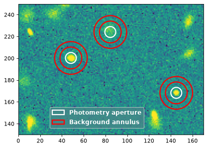
We perform aperture photometry for three sources using circular apertures with a radius of 5 pixels. The local background is estimated from circular annuli with an inner radius of 10 pixels and an outer radius of 15 pixels. First, define the source and background apertures:

>>> from photutils.aperture import CircularAnnulus, CircularAperture
>>> positions = [(145.1, 168.3), (84.5, 224.1), (48.3, 200.3)]
>>> aperture = CircularAperture(positions, r=5)
>>> annulus_aperture = CircularAnnulus(positions, r_in=10, r_out=15)

The following figure shows the source apertures (white) and background annuli (red) overlaid on a cutout containing the three sources:

(Source code, png, hires.png, pdf, svg)

Simple mean within a circular annulus#

We first use the ApertureStats class to compute the mean background level within the annulus at each source position:

>>> from photutils.aperture import ApertureStats
>>> aperstats = ApertureStats(data, annulus_aperture)
>>> bkg_mean = aperstats.mean
>>> print(bkg_mean)
[4.99411764 5.1349344  4.86894665]

Next, we use AperturePhotometry to measure the source fluxes in the circular apertures:

>>> from photutils.aperture import AperturePhotometry
>>> phot = AperturePhotometry(data, aperture, error=error)
>>> phot_table = phot.to_table()
>>> for col in phot_table.colnames:
...     phot_table[col].info.format = '%.8g'  # for consistent table output
>>> phot_table.pprint(max_width=-1)
 id x_center y_center    flux    flux_err     area   flags
                                              pix2
--- -------- -------- --------- ---------- --------- -----
  1    145.1    168.3 1128.1245  0.8552501 78.539816     0
  2     84.5    224.1   735.739 0.85778957 78.539816     0
  3     48.3    200.3 1299.6341 0.85681906 78.539816     0

The total background within each source aperture is the mean background per pixel multiplied by the aperture area. Rather than the analytical aperture area, use the unmasked overlap area that was actually used for the photometry, which is available in the 'area' column of the output table above (equivalent to the area_overlap() method computed with the same photometry inputs). Using this computed area ensures the background is scaled consistently with the photometry, correctly accounting for the overlap method and any masked pixels:

>>> aperture_area = phot_table['area'].value
>>> total_bkg = bkg_mean * aperture_area
>>> print(total_bkg)
[392.23708187 403.29680431 382.40617607]

Subtracting this background estimate from the measured aperture sums gives the background-subtracted photometry:

>>> phot_bkgsub = phot_table['flux'] - total_bkg

Finally, we add the local background estimate, the total background within the aperture, and the background-subtracted photometry to the output table:

>>> phot_table['total_bkg'] = total_bkg
>>> phot_table['flux_bkgsub'] = phot_bkgsub
>>> for col in phot_table.colnames:
...     phot_table[col].info.format = '%.8g'  # for consistent table output
>>> phot_table.pprint(max_width=-1)
 id x_center y_center    flux    flux_err     area   flags total_bkg flux_bkgsub
                                              pix2
--- -------- -------- --------- ---------- --------- ----- --------- -----------
  1    145.1    168.3 1128.1245  0.8552501 78.539816     0 392.23708   735.88739
  2     84.5    224.1   735.739 0.85778957 78.539816     0  403.2968   332.44219
  3     48.3    200.3 1299.6341 0.85681906 78.539816     0 382.40618   917.22792

Sigma-clipped median within a circular annulus#

In this example, the local background is estimated as the sigma-clipped median within each circular annulus. We use ApertureStats to compute both the source photometry and the local background:

>>> from astropy.stats import SigmaClip
>>> sigclip = SigmaClip(sigma=3.0, maxiters=10)
>>> aper_stats = ApertureStats(data, aperture, sigma_clip=None)
>>> bkg_stats = ApertureStats(data, annulus_aperture, sigma_clip=sigclip)
>>> total_bkg = bkg_stats.median * aper_stats.sum_aper_area.value
>>> apersum_bkgsub = aper_stats.sum - total_bkg
>>> print(apersum_bkgsub)
[743.77088731 338.59823118 920.07553956]

If you want to compute additional source properties on the background-subtracted data (not just sum), pass the per-pixel local background values to ApertureStats using the local_bkg keyword. The local background is then subtracted internally when computing all source properties:

>>> aper_stats_bkgsub = ApertureStats(data, aperture,
...                                   local_bkg=bkg_stats.median)
>>> print(aper_stats_bkgsub.sum)
[743.77088731 338.59823118 920.07553956]

The resulting aperture sums are identical to those computed above.

Aperture Masks#

All PixelAperture classes provide a to_mask() method that returns an ApertureMask for a single aperture position, or a list of ApertureMask objects when the aperture has multiple positions. Each ApertureMask contains the aperture mask weights together with a BoundingBox that defines where the mask should be applied to an image.

We begin by creating a circular annulus aperture:

>>> from photutils.aperture import CircularAnnulus
>>> from photutils.datasets import make_100gaussians_image
>>> data = make_100gaussians_image()
>>> positions = [(145.1, 168.3), (84.5, 224.1), (48.3, 200.3)]
>>> aperture = CircularAnnulus(positions, r_in=10, r_out=15)

Next, we create the corresponding ApertureMask objects using the to_mask() method with the 'exact' overlap method:

>>> masks = aperture.to_mask(method='exact')

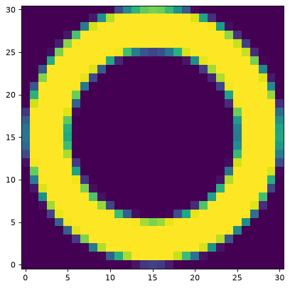
The following figure shows the first aperture mask:

>>> import matplotlib.pyplot as plt
>>> fig, ax = plt.subplots()
>>> ax.imshow(masks[0], origin='lower')

(Source code, png, hires.png, pdf, svg)

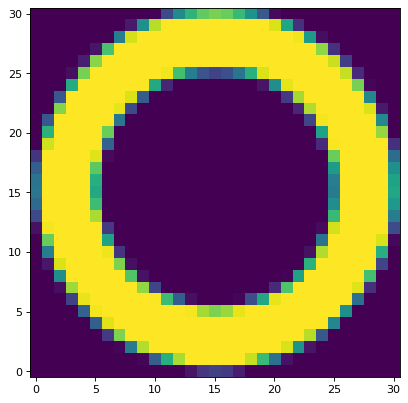
Now create a mask using the 'center' overlap method and plot the result:

>>> masks2 = aperture.to_mask(method='center')
>>> fig, ax = plt.subplots()
>>> ax.imshow(masks2[0], origin='lower')

(Source code, png, hires.png, pdf, svg)

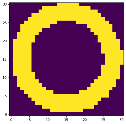
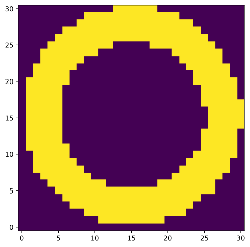
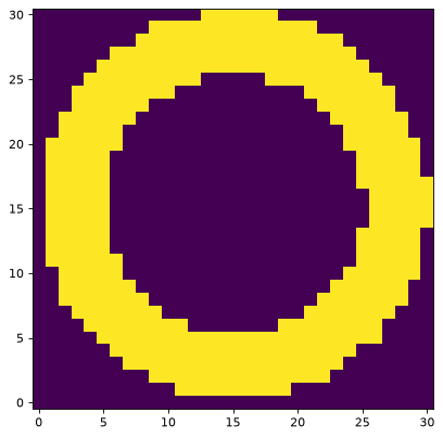
The 'center' method produces a binary mask, in contrast to the fractional weights returned by the 'exact' method.

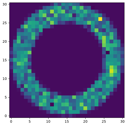
We can also use an ApertureMask to create a mask-weighted cutout from the data, with partial or non-overlapping regions handled automatically. The following example plots the first cutout using the mask generated above with the 'exact' overlap method:

>>> data_weighted = masks[0].multiply(data)
>>> fig, ax = plt.subplots()
>>> ax.imshow(data_weighted, origin='lower')

(Source code, png, hires.png, pdf, svg)

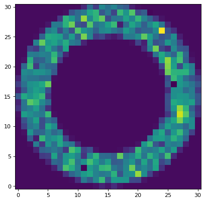
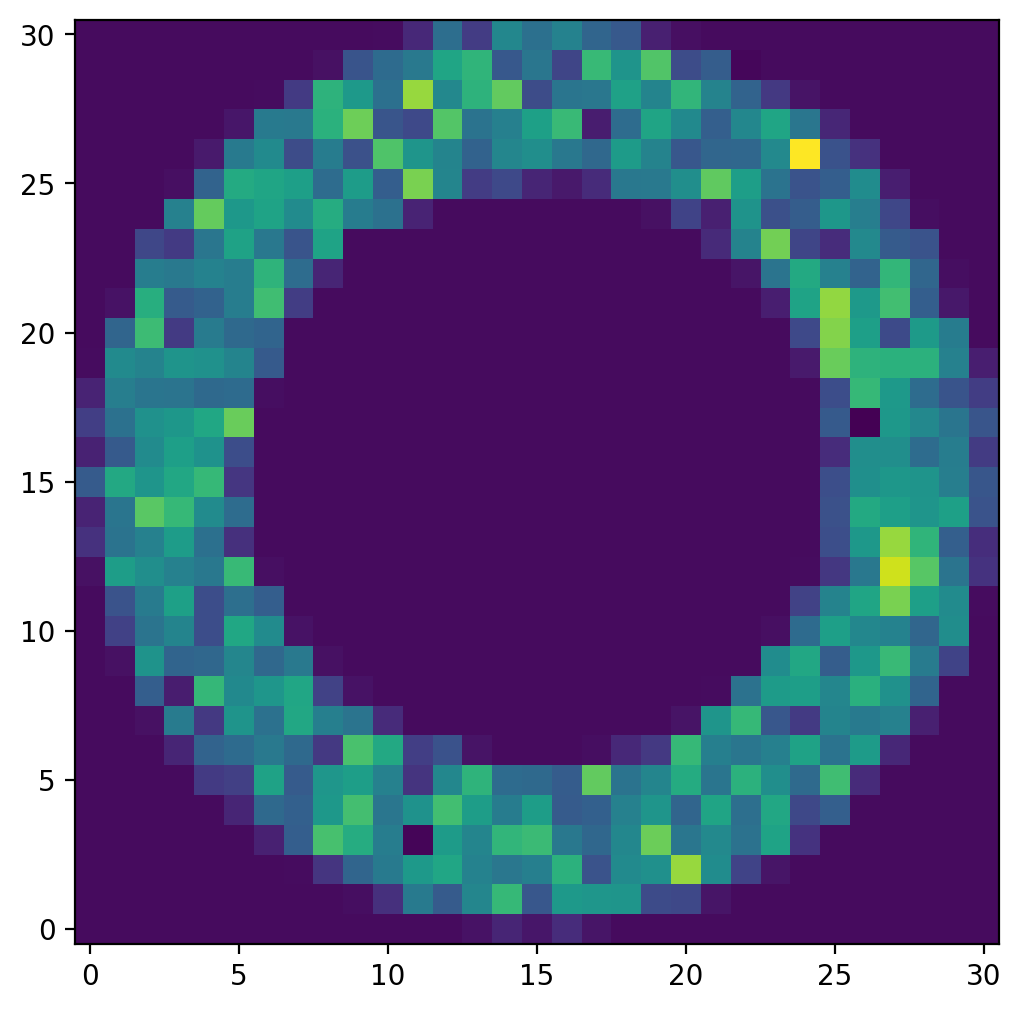
To obtain a one-dimensional ndarray containing the non-zero, mask-weighted data values, use the get_values() method:

>>> data_weighted_1d = masks[0].get_values(data)

The ApertureMask class also provides a to_image() method to create a 2D image of the mask with a specified shape, and a cutout() method to extract a cutout of the input data over the mask bounding box. Both methods automatically handle cases where the mask partially overlaps or lies completely outside the input data.

Together, these methods provide convenient access to both the aperture mask itself and the corresponding regions of the input data.

API Reference#

Aperture Photometry (photutils.aperture)

Aperture Photometry (photutils.aperture)#

Introduction#

Apertures#

Creating Aperture Objects#

Converting Between Pixel and Sky Apertures#

Polygon Apertures#

Converting to Polygon Apertures#

Performing Aperture Photometry#

Aperture and Pixel Overlap#

Aperture Photometry Error Estimation#

Aperture Photometry with Multiple Apertures at Each Position#

Aperture Photometry on a 3D Data Cube#

Masking Pixels in Aperture Photometry#

Masking Bad Pixels#

Masking Neighboring Sources with a Segmentation Image#

Aperture Quality Flags#

Aperture Statistics#

Background Subtraction#

Global Background Subtraction#

Local Background Subtraction#

Simple mean within a circular annulus#

Sigma-clipped median within a circular annulus#

Aperture Masks#

API Reference#

Aperture Photometry (`photutils.aperture`)#