CurveOfGrowth

class photutils.profiles.CurveOfGrowth(data, xycen, radii, *, error=None, mask=None, method='exact', subpixels=5)

Bases: ProfileBase

Class to create a curve of growth using concentric circular apertures.

The curve of growth profile represents the circular aperture flux as a function of circular radius.

Parameters:

data2D ndarray

The 2D data array. The data should be background-subtracted. Non-finite values (e.g., NaN or inf) in the data or error array are automatically masked.

xycentuple of 2 floats

The (x, y) pixel coordinate of the source center.

radii1D float ndarray

An array of the circular radii. radii must be strictly increasing with a minimum value greater than zero, and contain at least 2 values. The radial spacing does not need to be constant.

error2D ndarray, optional

The 1-sigma errors of the input data. error is assumed to include all sources of error, including the Poisson error of the sources (see calc_total_error) . error must have the same shape as the input data. Non-finite values (e.g., NaN or inf) in the data or error array are automatically masked.

mask2D bool ndarray, optional

A boolean mask with the same shape as data where a True value indicates the corresponding element of data is masked. Masked data are excluded from all calculations.

method{‘exact’, ‘center’, ‘subpixel’}, optional

The method used to determine the overlap of the aperture on the pixel grid:

• 'exact' (default): The exact fractional overlap of the aperture and each pixel is calculated. The aperture weights will contain values between 0 and 1.

• 'center': A pixel is considered to be entirely in or out of the aperture depending on whether its center is in or out of the aperture. The aperture weights will contain values only of 0 (out) and 1 (in).

• 'subpixel': A pixel is divided into subpixels (see the subpixels keyword), each of which are considered to be entirely in or out of the aperture depending on whether its center is in or out of the aperture. If subpixels=1, this method is equivalent to 'center'. The aperture weights will contain values between 0 and 1.

subpixelsint, optional

For the 'subpixel' method, resample pixels by this factor in each dimension. That is, each pixel is divided into subpixels**2 subpixels. This keyword is ignored unless method='subpixel'.

Examples

>>> import numpy as np
>>> from astropy.modeling.models import Gaussian2D
>>> from astropy.visualization import simple_norm
>>> from photutils.centroids import centroid_quadratic
>>> from photutils.datasets import make_noise_image
>>> from photutils.profiles import CurveOfGrowth

Create an artificial single source. Note that this image does not have any background.

>>> gmodel = Gaussian2D(42.1, 47.8, 52.4, 4.7, 4.7, 0)
>>> yy, xx = np.mgrid[0:100, 0:100]
>>> data = gmodel(xx, yy)
>>> error = make_noise_image(data.shape, mean=0., stddev=2.4, seed=123)
>>> data += error

Create the curve of growth.

>>> xycen = centroid_quadratic(data, xpeak=48, ypeak=52)
>>> radii = np.arange(1, 26)
>>> cog = CurveOfGrowth(data, xycen, radii, error=error, mask=None)

>>> print(cog.radius)  
[ 1  2  3  4  5  6  7  8  9 10 11 12 13 14 15 16 17 18 19 20 21 22 23 24
 25]

>>> print(cog.profile)  
[ 130.57472018  501.34744442 1066.59182074 1760.50163608 2502.13955554
 3218.50667597 3892.81448231 4455.36403436 4869.66609313 5201.99745378
 5429.02043984 5567.28370644 5659.24831854 5695.06577065 5783.46217755
 5824.01080702 5825.59003768 5818.22316662 5866.52307412 5896.96917375
 5948.92254787 5968.30540534 5931.15611704 5941.94457249 5942.06535486]

>>> print(cog.profile_error)  
[  5.32777186   9.37111012  13.41750992  16.62928904  21.7350922
  25.39862532  30.3867526   34.11478867  39.28263973  43.96047829
  48.11931395  52.00967328  55.7471834   60.48824739  64.81392778
  68.71042311  72.71899201  76.54959872  81.33806741  85.98568713
  91.34841248  95.5173253   99.22190499 102.51980185 106.83601366]

Plot the curve of growth.

(Source code, png, hires.png, pdf, svg)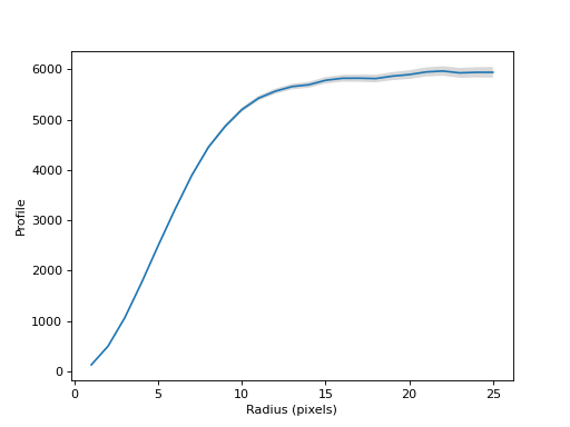

Normalize the profile and plot the normalized curve of growth.

(Source code, png, hires.png, pdf, svg)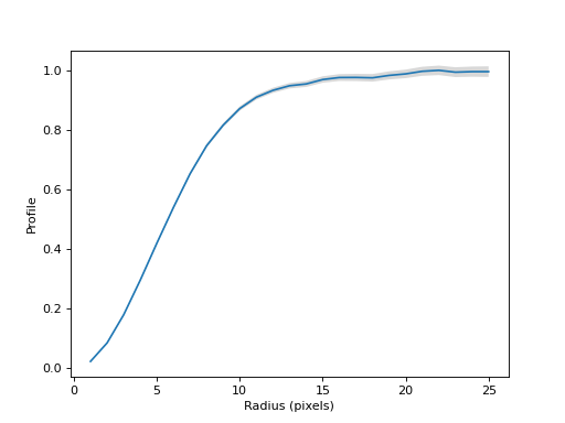

Plot a couple of the apertures on the data.

(Source code, png, hires.png, pdf, svg)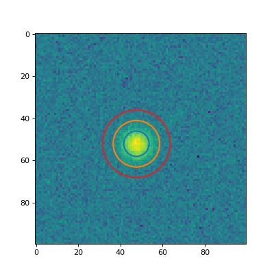

Attributes Summary

apertures	A list of CircularAperture objects used to measure the profile.
area	The unmasked area in each circular aperture as a function of radius as a 1D ndarray.
profile	The curve-of-growth profile as a 1D ndarray.
profile_error	The curve-of-growth profile errors as a 1D ndarray.
radius	The profile radius in pixels as a 1D ndarray.

Methods Summary

calc_ee_at_radius(radius)	Calculate the encircled energy at a given radius using a cubic interpolator based on the profile data.
calc_radius_at_ee(ee)	Calculate the radius at a given encircled energy using a cubic interpolator based on the profile data.
normalize([method])	Normalize the profile.
plot([ax])	Plot the profile.
plot_error([ax])	Plot the profile errors.
unnormalize()	Unnormalize the profile back to the original state before any calls to normalize.

Attributes Documentation

apertures

A list of CircularAperture objects used to measure the profile.

If radius_min is zero, then the first item will be None.

area

The unmasked area in each circular aperture as a function of radius as a 1D ndarray.

profile

The curve-of-growth profile as a 1D ndarray.

profile_error

The curve-of-growth profile errors as a 1D ndarray.

radius

The profile radius in pixels as a 1D ndarray.

This is the same as the input radii.

Note that these are the radii of the circular apertures used to measure the profile. Thus, they are the radial values that enclose the given flux. They can be used directly to measure the encircled energy/flux at a given radius.

Methods Documentation

calc_ee_at_radius(radius)

Calculate the encircled energy at a given radius using a cubic interpolator based on the profile data.

Note that this function assumes that input data has been normalized such that the total enclosed flux is 1 for an infinitely large radius. You can also use the normalize method before calling this method to normalize the profile to be 1 at the largest input radii.

Parameters:

radiusfloat or 1D ndarray

The circular radius/radii.

Returns:

eendarray

The encircled energy at each radius/radii. Returns NaN for radii outside the range of the profile data.

calc_radius_at_ee(ee)

Calculate the radius at a given encircled energy using a cubic interpolator based on the profile data.

Note that this function assumes that input data has been normalized such that the total enclosed flux is 1 for an infinitely large radius. You can also use the normalize method before calling this method to normalize the profile to be 1 at the largest input radii.

This interpolator returns values only for regions where the curve-of-growth profile is monotonically increasing.

Parameters:

eefloat or 1D ndarray

The encircled energy.

Returns:

radiusndarray

The radius at each encircled energy. Returns NaN for encircled energies outside the range of the profile data.

normalize(method='max')

Normalize the profile.

Parameters:

method{‘max’, ‘sum’}, optional

The method used to normalize the profile:

• 'max' (default): The profile is normalized such that its maximum value is 1.

• 'sum': The profile is normalized such that its sum (integral) is 1.

plot(ax=None, **kwargs)

Plot the profile.

Parameters:

axmatplotlib.axes.Axes or None, optional

The matplotlib axes on which to plot. If None, then the current Axes instance is used.

**kwargsdict, optional

Any keyword arguments accepted by matplotlib.pyplot.plot.

Returns:

lineslist of Line2D

A list of lines representing the plotted data.

plot_error(ax=None, **kwargs)

Plot the profile errors.

Parameters:

axmatplotlib.axes.Axes or None, optional

The matplotlib axes on which to plot. If None, then the current Axes instance is used.

**kwargsdict, optional

Any keyword arguments accepted by matplotlib.pyplot.fill_between.

Returns:

linesmatplotlib.collections.PolyCollection

A PolyCollection containing the plotted polygons.

unnormalize()

Unnormalize the profile back to the original state before any calls to normalize.