Profiles (photutils.profiles)

Introduction

photutils.profiles provides tools to calculate radial profiles and curves of growth using concentric circular apertures.

Preliminaries

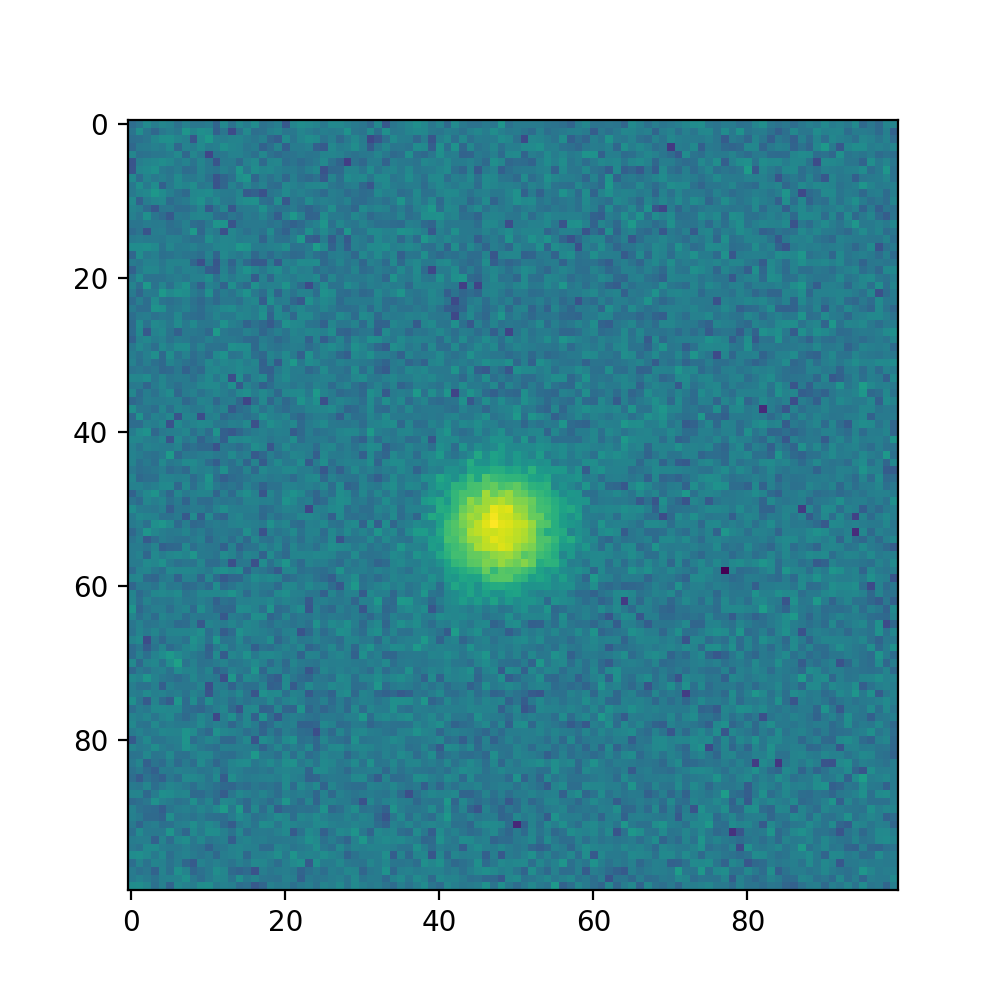
Let’s start by making a synthetic image of a single source. Note that there is no background in this image. One should background-subtract the data before creating a radial profile or curve of growth.

>>> import numpy as np
>>> from astropy.modeling.models import Gaussian2D
>>> from photutils.datasets import make_noise_image

>>> gmodel = Gaussian2D(42.1, 47.8, 52.4, 4.7, 4.7, 0)
>>> yy, xx = np.mgrid[0:100, 0:100]
>>> data = gmodel(xx, yy)
>>> error = make_noise_image(data.shape, mean=0., stddev=2.4, seed=123)
>>> data += error

(Source code, png, hires.png, pdf, svg)

Creating a Radial Profile

Photutils provides the RadialProfile class for computing radial profiles. The radial bins are defined by inputting a 1D array of radial edges. The radial spacing does not need to be constant.

First, we’ll use the centroid_quadratic function to find the source centroid:

>>> from photutils.centroids import centroid_quadratic
>>> xycen = centroid_quadratic(data, xpeak=48, ypeak=52)
>>> print(xycen)  
[47.61226319 52.04668132]

Now, let’s create a radial profile. The radial profile will be centered at our centroid position computed above.

>>> from photutils.profiles import RadialProfile
>>> edge_radii = np.arange(25)
>>> rp = RadialProfile(data, xycen, edge_radii, error=error, mask=None)

The radius (radial bin centers), profile, and profile_error attributes contain the output 1D ndarray objects:

>>> print(rp.radius)  
[ 0.5  1.5  2.5  3.5  4.5  5.5  6.5  7.5  8.5  9.5 10.5 11.5 12.5 13.5
 14.5 15.5 16.5 17.5 18.5 19.5 20.5 21.5 22.5 23.5]

>>> print(rp.profile)  
[ 4.15632243e+01  3.93402079e+01  3.59845746e+01  3.15540506e+01
  2.62300757e+01  2.07297033e+01  1.65106801e+01  1.19376723e+01
  7.75743772e+00  5.56759777e+00  3.44112671e+00  1.91350281e+00
  1.17092981e+00  4.22261078e-01  9.70256904e-01  4.16355795e-01
  1.52328707e-02 -6.69985111e-02  4.15522650e-01  2.48494731e-01
  4.03348112e-01  1.43482678e-01 -2.62777461e-01  7.30653622e-02]

>>> print(rp.profile_error)  
[1.69588246 0.81797694 0.61132694 0.44670831 0.49499835 0.38025361
 0.40844702 0.32906672 0.36466713 0.33059274 0.29661894 0.27314739
 0.25551933 0.27675376 0.25553986 0.23421017 0.22966813 0.21747036
 0.23654884 0.22760386 0.23941711 0.20661313 0.18999134 0.17469024]

If desired, the radial profiles can be normalized using the normalize() method.

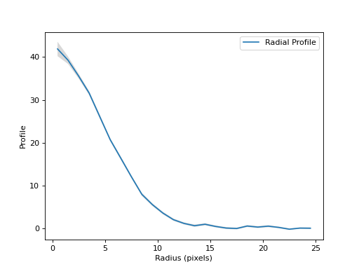
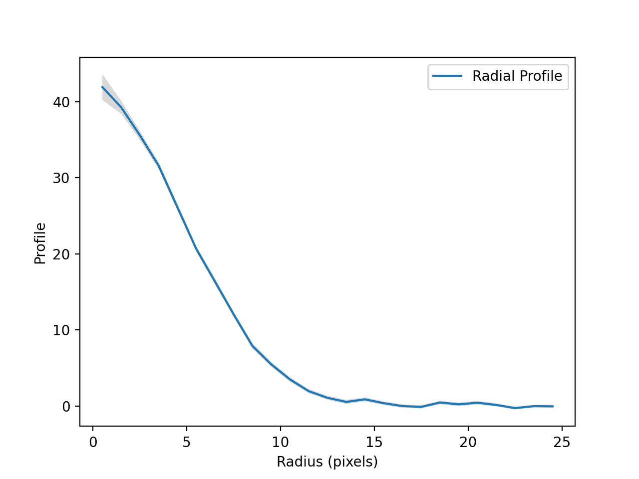
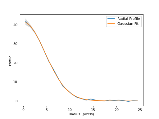
There are also convenience methods to plot the radial profile and its error:

>>> rp.plot(label='Radial Profile')
>>> rp.plot_error()

(Source code, png, hires.png, pdf, svg)

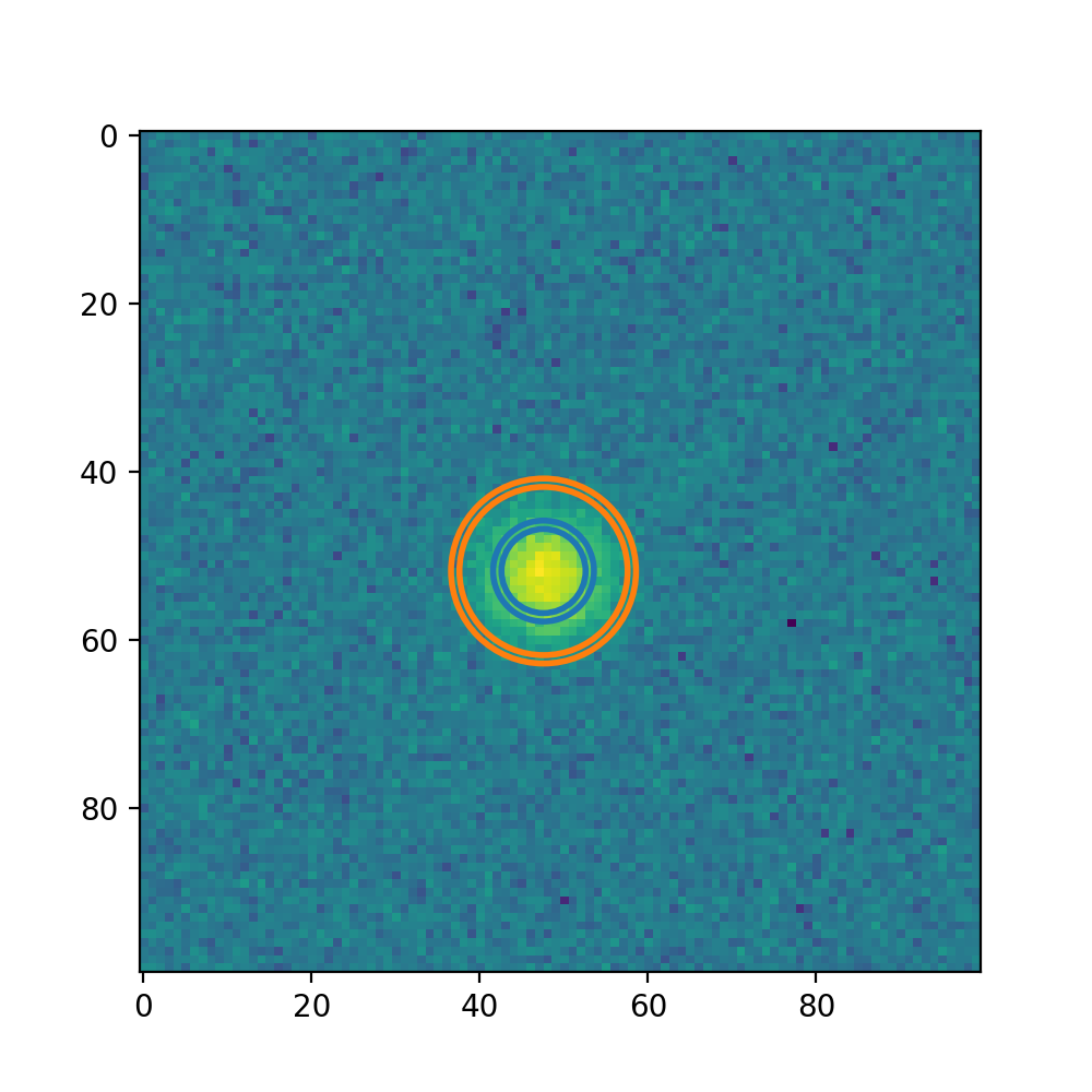
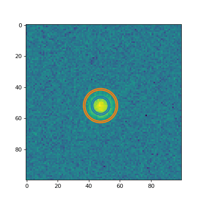
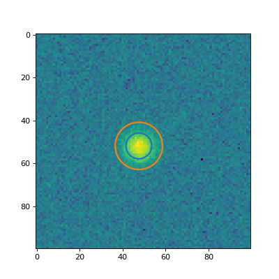
The apertures attribute contains a list of the apertures. Let’s plot two of the annulus apertures for the RadialProfile instance on the data:

(Source code, png, hires.png, pdf, svg)

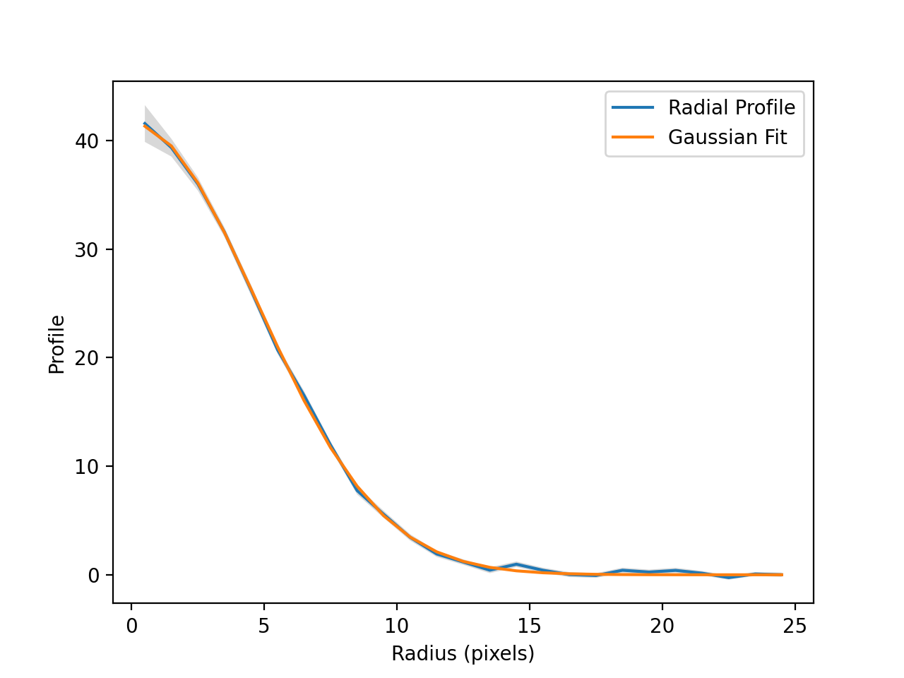
Now let’s fit a 1D Gaussian to the radial profile and return the Gaussian model using the gaussian_fit attribute:

>>> rp.gaussian_fit  
<Gaussian1D(amplitude=41.54880743, mean=0., stddev=4.71059406)>

The FWHM of the fitted 1D Gaussian model is stored in the gaussian_fwhm attribute:

>>> print(rp.gaussian_fwhm)  
11.09260130738712

Finally, let’s plot the fitted 1D Gaussian model for the class:RadialProfile radial profile:

(Source code, png, hires.png, pdf, svg)

Creating a Curve of Growth

Now let’s create a curve of growth using the CurveOfGrowth class. We use the simulated image defined above and the same source centroid.

The curve of growth will be centered at our centroid position. It will be computed over the radial range given by the input radii array:

>>> from photutils.profiles import CurveOfGrowth
>>> radii = np.arange(1, 26)
>>> cog = CurveOfGrowth(data, xycen, radii, error=error, mask=None)

The CurveOfGrowth instance has radius, profile, and profile_error attributes which contain 1D ndarray objects:

>>> print(cog.radius)  
[ 1  2  3  4  5  6  7  8  9 10 11 12 13 14 15 16 17 18 19 20 21 22 23 24
 25]

>>> print(cog.profile)  
[ 130.57472018  501.34744442 1066.59182074 1760.50163608 2502.13955554
 3218.50667597 3892.81448231 4455.36403436 4869.66609313 5201.99745378
 5429.02043984 5567.28370644 5659.24831854 5695.06577065 5783.46217755
 5824.01080702 5825.59003768 5818.22316662 5866.52307412 5896.96917375
 5948.92254787 5968.30540534 5931.15611704 5941.94457249 5942.06535486]

>>> print(cog.profile_error)  
[  5.32777186   9.37111012  13.41750992  16.62928904  21.7350922
  25.39862532  30.3867526   34.11478867  39.28263973  43.96047829
  48.11931395  52.00967328  55.7471834   60.48824739  64.81392778
  68.71042311  72.71899201  76.54959872  81.33806741  85.98568713
  91.34841248  95.5173253   99.22190499 102.51980185 106.83601366]

If desired, the curve of growth profile can be normalized using the normalize() method.

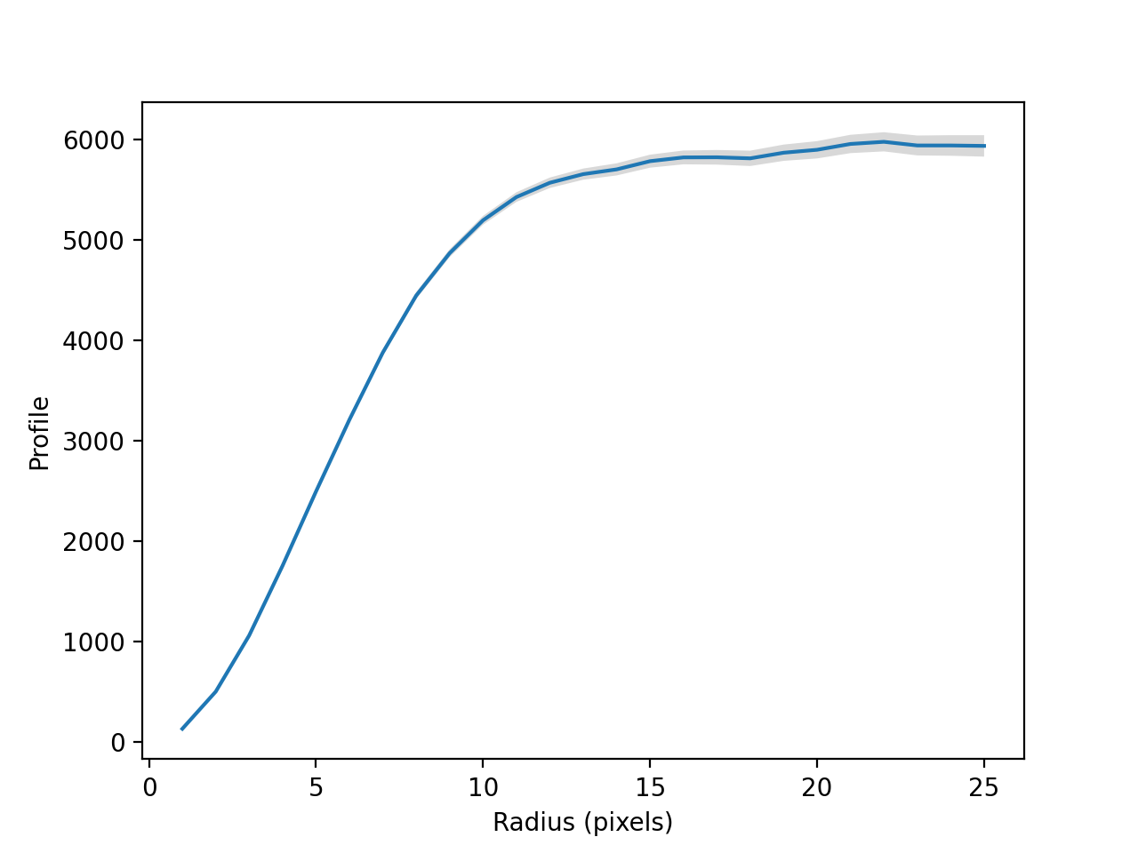
There are also convenience methods to plot the curve of growth and its error:

>>> rp.plot()
>>> rp.plot_error()

(Source code, png, hires.png, pdf, svg)

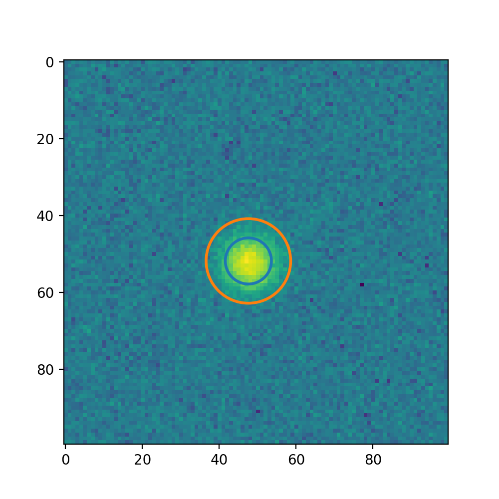
The apertures attribute contains a list of the apertures. Let’s plot a couple of the apertures on the data:

(Source code, png, hires.png, pdf, svg)

Reference/API

This subpackage contains tools for generating radial profiles.

Classes

CurveOfGrowth(data, xycen, radii, *[, ...])	Class to create a curve of growth using concentric circular apertures.
ProfileBase(data, xycen, radii, *[, error, ...])	Abstract base class for profile classes.
RadialProfile(data, xycen, radii, *[, ...])	Class to create a radial profile using concentric circular apertures.

Class Inheritance Diagram