PSF Photometry (photutils.psf)

The photutils.psf subpackage contains tools for model-fitting photometry, often called “PSF photometry”.

Terminology

Different astronomy subfields use the terms “PSF”, “PRF”, or related terms somewhat differently, especially when colloquial usage is taken into account. This package aims to be at the very least internally consistent, following the definitions described here.

We take the Point Spread Function (PSF), or instrumental Point Spread Function (iPSF) to be the infinite-resolution and infinite-signal-to-noise flux distribution from a point source on the detector, after passing through optics, dust, atmosphere, etc. By contrast, the function describing the responsivity variations across individual pixels is the Pixel Response Function (sometimes called “PRF”, but that acronym is not used here for reasons that will soon be apparent). The convolution of the PSF and pixel response function, when discretized onto the detector (i.e., a rectilinear CCD grid), is the effective PSF (ePSF) or Point Response Function (PRF) (this latter terminology is the definition used by Spitzer). In many cases the PSF/ePSF/PRF distinction is unimportant, and the ePSF/PRF are simply called the “PSF”, but the distinction can be critical when dealing carefully with undersampled data or detectors with significant intra-pixel sensitivity variations. For a more detailed description of this formalism, see Anderson & King 2000.

All this said, in colloquial usage “PSF photometry” sometimes refers to the more general task of model-fitting photometry (with the effects of the PSF either implicitly or explicitly included in the models), regardless of exactly what kind of model is actually being fit. For brevity (e.g., photutils.psf), we use “PSF photometry” in this way, as a shorthand for the general approach.

PSF Photometry

Photutils provides a modular set of tools to perform PSF photometry for different science cases. The tools are implemented as classes that perform various subtasks of PSF photometry. High-level classes are also provided to connect these pieces together.

The two main PSF-photometry classes are PSFPhotometry and IterativePSFPhotometry. PSFPhotometry provides the framework for a flexible PSF photometry workflow that can find sources in an image, optionally group overlapping sources, fit the PSF model to the sources, and subtract the fit PSF models from the image. IterativePSFPhotometry is an iterative version of PSFPhotometry where after the fit sources are subtracted, the process repeats until no additional sources are detected or a maximum number of iterations has been reached. When used with the DAOStarFinder, IterativePSFPhotometry is essentially an implementation of the DAOPHOT algorithm described by Stetson in his seminal paper for crowded-field stellar photometry.

The star-finding step is controlled by the finder keyword, where one inputs a callable function or class instance. Typically, this would be one of the star-detection classes implemented in the photutils.detection subpackage, e.g., DAOStarFinder, IRAFStarFinder, or StarFinder.

After finding sources, one can optionally apply a clustering algorithm to group overlapping sources using the grouper keyword. Usually, groups are formed by a distance criterion, which is the case of the grouping algorithm proposed by Stetson. Stars that grouped are fit simultaneously. The reason behind the construction of groups and not fitting all stars simultaneously is illustrated as follows: imagine that one would like to fit 300 stars and the model for each star has three parameters to be fitted. If one constructs a single model to fit the 300 stars simultaneously, then the optimization algorithm will have to search for the solution in a 900-dimensional space, which is computationally expensive and error-prone. Having smaller groups of stars effectively reduces the dimension of the parameter space, which facilitates the optimization process. For more details see Source Grouping Algorithms.

The local background around each source can optionally be subtracted using the localbkg_estimator keyword. This keyword accepts a LocalBackground instance that estimates the local statistics in a circular annulus aperture centered on each source. The size of the annulus and the statistic function can be configured in LocalBackground.

The next step is to fit the sources and/or groups. This task is performed using an astropy fitter, for example LevMarLSQFitter, input via the fitter keyword. The shape of the region to be fitted can be configured using the fit_shape parameter. In general, fit_shape should be set to a small size (e.g., (5, 5)) that covers the central star region with the highest flux signal-to-noise. The initial positions are derived from the finder algorithm. The initial flux values for the fit are derived from measuring the flux in a circular aperture with radius aperture_radius. The initial positions and fluxes can be alternatively input in a table via the init_params keyword when calling the class.

After sources are fitted, a model image of the fit sources or a residual image can be generated using the make_model_image() and make_residual_image() methods, respectively.

For IterativePSFPhotometry, the above steps can be repeated until no additional sources are detected (or until a maximum number of iterations).

The PSFPhotometry and IterativePSFPhotometry classes provide the structure in which the PSF-fitting steps described above are performed, but all the stages can be turned on or off or replaced with different implementations as the user desires. This makes the tools very flexible. One can also bypass several of the steps by directly inputting to init_params an astropy table containing the initial parameters for the source centers, fluxes, group identifiers, and local backgrounds. This is also useful if one is interested in fitting only one or a few sources in an image.

Example Usage

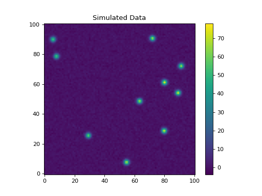
Let’s start with a simple example using simulated stars whose PSF is assumed to be Gaussian. We’ll create a synthetic image using tools provided by the photutils.datasets module:

>>> import numpy as np
>>> from photutils.datasets import make_test_psf_data, make_noise_image
>>> from photutils.psf import IntegratedGaussianPRF
>>> psf_model = IntegratedGaussianPRF(flux=1, sigma=2.7 / 2.35)
>>> psf_shape = (9, 9)
>>> nsources = 10
>>> shape = (101, 101)
>>> data, true_params = make_test_psf_data(shape, psf_model, psf_shape,
...                                        nsources, flux_range=(500, 700),
...                                        min_separation=10, seed=0)
>>> noise = make_noise_image(data.shape, mean=0, stddev=1, seed=0)
>>> data += noise
>>> error = np.abs(noise)

Let’s plot the image:

(Source code, png, hires.png, pdf, svg)

Fitting multiple stars

Now let’s use PSFPhotometry to perform PSF photometry on the stars in this image. Note that the input image must be background-subtracted prior to using the photometry classes. See Background Estimation (photutils.background) for tools to subtract a global background from an image. This is not needed for our synthetic image because it does not include background.

We’ll use the DAOStarFinder class for source detection. We’ll estimate the initial fluxes of each source using a circular aperture with a radius 4 pixels. The central 5x5 pixel region of each star will be fit using an IntegratedGaussianPRF PSF model. First, let’s create an instance of the PSFPhotometry class:

>>> from photutils.detection import DAOStarFinder
>>> from photutils.psf import PSFPhotometry
>>> psf_model = IntegratedGaussianPRF(flux=1, sigma=2.7 / 2.35)
>>> fit_shape = (5, 5)
>>> finder = DAOStarFinder(6.0, 2.0)
>>> psfphot = PSFPhotometry(psf_model, fit_shape, finder=finder,
...                         aperture_radius=4)

To perform the PSF fitting, we then call the class instance on the data array, and optionally an error and mask array. A NDData object holding the data, error, and mask arrays can also be input into the data parameter. Note that all non-finite (e.g., NaN or inf) data values are automatically masked. Here we input the data and error arrays:

>>> phot = psfphot(data, error=error)

A table of initial PSF model parameter values can also be input when calling the class instance. An example of that is shown later.

Equivalently, one can input an NDData object with any uncertainty object that can be converted to standard-deviation errors:

>>> from astropy.nddata import NDData, StdDevUncertainty
>>> uncertainty = StdDevUncertainty(error)
>>> nddata = NDData(data, uncertainty=uncertainty)
>>> phot2 = psfphot(nddata)

The result is an astropy Table with columns for the source and group identification numbers, the x, y, and flux initial, fit, and error values, local background, number of unmasked pixels fit, the group size, quality-of-fit metrics, and flags. See the PSFPhotometry documentation for descriptions of the output columns.

The full table cannot be shown here as it has many columns, but let’s print the source ID along with the fit x, y, and flux values:

>>> phot['x_fit'].info.format = '.4f'  # optional format
>>> phot['y_fit'].info.format = '.4f'
>>> phot['flux_fit'].info.format = '.4f'
>>> print(phot[('id', 'x_fit', 'y_fit', 'flux_fit')])  
 id  x_fit   y_fit  flux_fit
--- ------- ------- --------
  1 54.5641  7.7650 645.4552
  2 29.0866 25.6111 553.0376
  3 79.6285 28.7488 665.8715
  4 63.2344 48.6406 626.7983
  5 88.8849 54.1203 681.9908
  6 79.8762 61.1380 686.3628
  7 90.9606 72.0860 610.5911
  8  7.8021 78.5730 509.3270
  9  5.5349 89.8869 503.9691
 10 71.8411 90.5841 621.1757

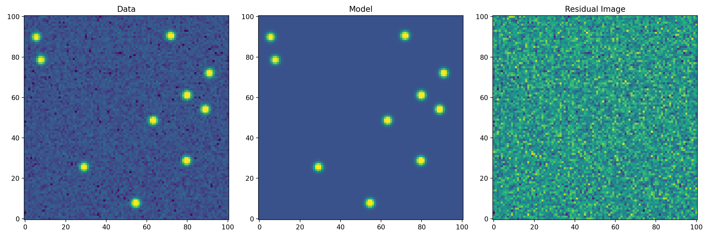
Let’s create the residual image:

>>> resid = psfphot.make_residual_image(data, (9, 9))

and plot it:

(Source code, png, hires.png, pdf, svg)

The residual image looks like noise, indicating good fits to the sources.

Further details about the PSF fitting can be obtained from attributes on the PSFPhotometry instance. For example, the results from the finder instance called during PSF fitting can be accessed using the finder_results attribute (the finder returns an astropy table):

>>> psfphot.finder_results['xcentroid'].info.format = '.4f'  # optional format
>>> psfphot.finder_results['ycentroid'].info.format = '.4f'  # optional format
>>> psfphot.finder_results['sharpness'].info.format = '.4f'  # optional format
>>> psfphot.finder_results['peak'].info.format = '.4f'
>>> psfphot.finder_results['flux'].info.format = '.4f'
>>> psfphot.finder_results['mag'].info.format = '.4f'
>>> print(psfphot.finder_results)  
 id xcentroid ycentroid sharpness ... sky   peak    flux    mag
--- --------- --------- --------- ... --- ------- ------- -------
  1   54.5300    7.7508    0.5996 ... 0.0 67.0314  8.7012 -2.3490
  2   29.0926   25.5993    0.5952 ... 0.0 58.7504  7.7484 -2.2230
  3   79.6189   28.7515    0.5956 ... 0.0 70.4621  9.2351 -2.4136
  4   63.2472   48.6151    0.5817 ... 0.0 64.9101  8.5701 -2.3325
  5   88.8827   54.1299    0.5954 ... 0.0 75.8880 10.3243 -2.5347
  6   79.8730   61.1214    0.6204 ... 0.0 78.0913 10.3346 -2.5357
  7   90.9621   72.0802    0.6162 ... 0.0 69.1417  9.2325 -2.4133
  8    7.7917   78.5454    0.5971 ... 0.0 52.7325  6.6840 -2.0626
  9    5.5845   89.8645    0.5721 ... 0.0 50.5544  6.5387 -2.0387
 10   71.8284   90.5625    0.6038 ... 0.0 65.7975  8.5373 -2.3283

The fit_results attribute contains a dictionary with a wealth of detailed information, including the fit models and any information returned from the fitter for each source:

>>> psfphot.fit_results.keys()
dict_keys(['local_bkg', 'init_params', 'fit_infos', 'fit_param_errs', 'fit_error_indices', 'npixfit', 'nmodels', 'psfcenter_indices', 'fit_residuals'])

As an example, let’s print the covariance matrix of the fit parameters for the first source (note that not all astropy fitters will return a covariance matrix):

>>> psfphot.fit_results['fit_infos'][0]['param_cov']  
array([[ 7.27034774e-01,  8.86845334e-04,  3.98593038e-03],
       [ 8.86845334e-04,  2.92871525e-06, -6.36805464e-07],
       [ 3.98593038e-03, -6.36805464e-07,  4.29520185e-05]])

Fitting a single source

In some cases, one may want to fit only a single source (or few sources) in an image. We can do that by defining a table of the sources that we want to fit. For this example, let’s fit the single star at (x, y) = (42, 36). We first define a table with this position and then pass that table into the init_params keyword when calling the PSF photometry class on the data:

>>> from astropy.table import QTable
>>> init_params = QTable()
>>> init_params['x'] = [63]
>>> init_params['y'] = [49]
>>> phot = psfphot(data, error=error, init_params=init_params)

The PSF photometry class allows for flexible input column names using a heuristic to identify the x, y, and flux columns. See PSFPhotometry for more details.

The output table contains only the fit results for the input source:

>>> phot['x_fit'].info.format = '.4f'  # optional format
>>> phot['y_fit'].info.format = '.4f'
>>> phot['flux_fit'].info.format = '.4f'
>>> print(phot[('id', 'x_fit', 'y_fit', 'flux_fit')])  
 id  x_fit   y_fit  flux_fit
--- ------- ------- --------
  1 63.2344 48.6406 626.7983

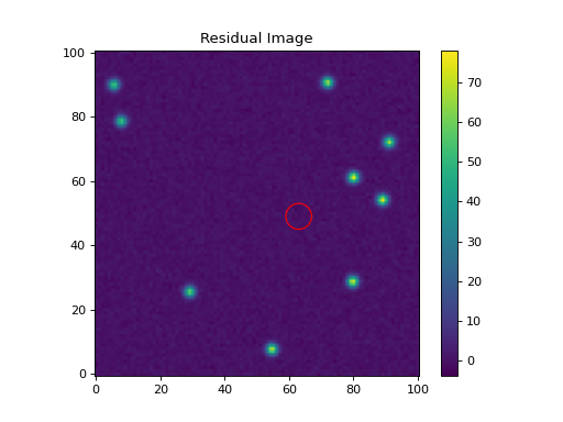
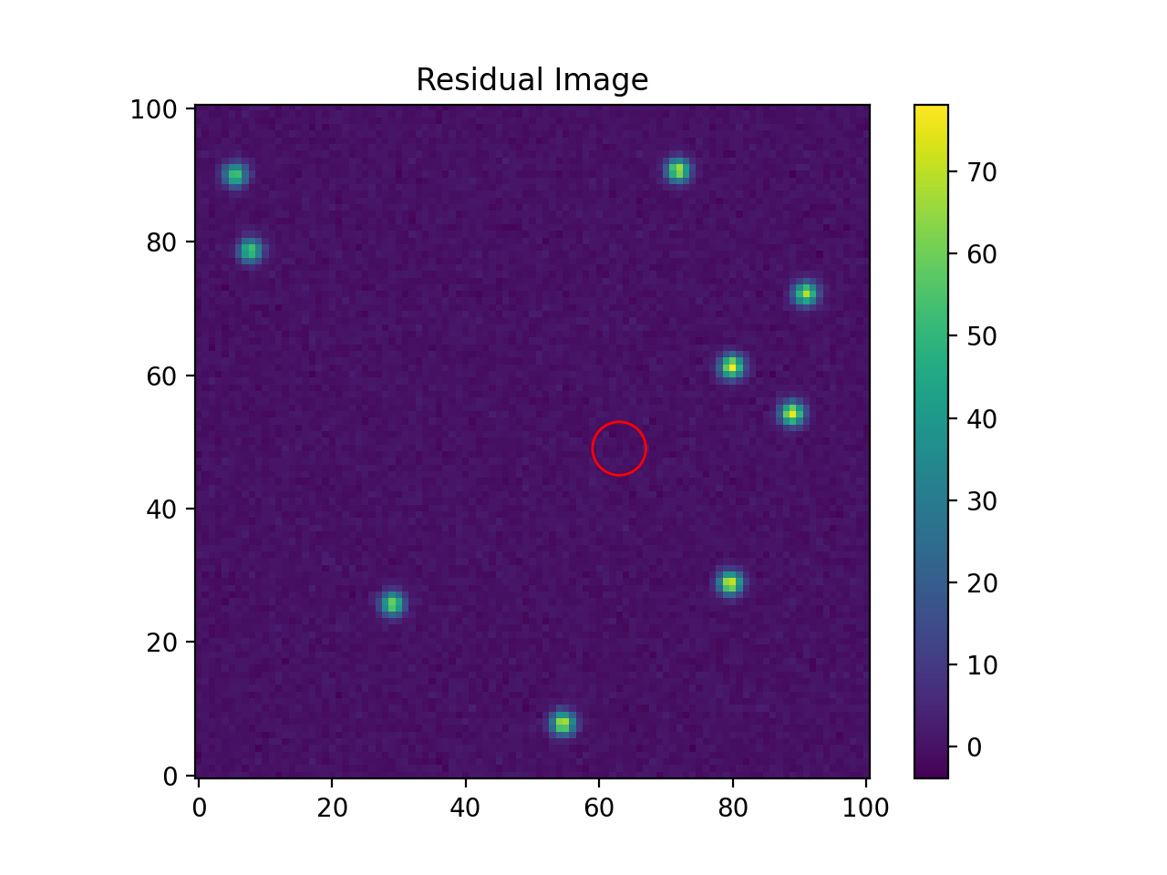
Finally, let’s show the residual image. The red circular aperture shows the location of the star that was fit and subtracted.

(Source code, png, hires.png, pdf, svg)

Forced Photometry

In general, the three parameters fit for each source are the x and y positions and the flux. However, the astropy modeling and fitting framework allows any of these parameters to be fixed during the fitting.

Let’s say you want to fix the (x, y) position for each source. You can do that by setting the fixed attribute on the model parameters:

>>> psf_model2 = IntegratedGaussianPRF(flux=1, sigma=2.7 / 2.35)
>>> psf_model2.x_0.fixed = True
>>> psf_model2.y_0.fixed = True
>>> psf_model2.fixed
{'flux': False, 'x_0': True, 'y_0': True, 'sigma': True}

Now when the model is fit, the flux will be varied but, the (x, y) position will be fixed at its initial position for every source. Let’s just fit a single source (defined in init_params):

>>> psfphot = PSFPhotometry(psf_model2, fit_shape, finder=finder,
...                         aperture_radius=4)
>>> phot = psfphot(data, error=error, init_params=init_params)

The output table shows that the (x, y) position was unchanged, with the fit values being identical to the initial values. However, the flux was fit:

>>> phot['flux_init'].info.format = '.4f'  # optional format
>>> phot['flux_fit'].info.format = '.4f'
>>> print(phot[('id', 'x_init', 'y_init', 'flux_init', 'x_fit',
...             'y_fit', 'flux_fit')])  
 id x_init y_init flux_init x_fit y_fit flux_fit
--- ------ ------ --------- ----- ----- --------
  1     63     49  619.5049  63.0  49.0 556.8463

Source Grouping

Source grouping is an optional feature. To turn it on, create a SourceGrouper instance and input it via the grouper keyword. Here we’ll group stars that are within 20 pixels of each other:

>>> from photutils.psf import SourceGrouper
>>> grouper = SourceGrouper(min_separation=20)
>>> psfphot = PSFPhotometry(psf_model, fit_shape, finder=finder,
...                         grouper=grouper, aperture_radius=4)
>>> phot = psfphot(data, error=error)

The group_id column shows that six groups were identified (each with two stars). The stars in each group were simultaneously fit.

>>> print(phot[('id', 'group_id', 'group_size')])
 id group_id group_size
--- -------- ----------
  1        1          1
  2        2          1
  3        3          1
  4        4          1
  5        5          3
  6        5          3
  7        5          3
  8        6          2
  9        6          2
 10        7          1

Care should be taken in defining the star groups. As noted above, simultaneously fitting very large star groups is computationally expensive and error-prone. A warning will be raised if the number of sources in a group exceeds 25.

Local Background Subtraction

To subtract a local background from each source, define a LocalBackground instance and input it via the localbkg_estimator keyword. Here we’ll use an annulus with an inner and outer radius of 5 and 10 pixels, respectively, with the MMMBackground statistic (with its default sigma clipping):

>>> from photutils.background import LocalBackground, MMMBackground
>>> bkgstat = MMMBackground()
>>> localbkg_estimator = LocalBackground(5, 10, bkgstat)
>>> finder = DAOStarFinder(10.0, 2.0)
>>> psfphot = PSFPhotometry(psf_model, fit_shape, finder=finder,
...                         grouper=grouper, aperture_radius=4,
...                         localbkg_estimator=localbkg_estimator)
>>> phot = psfphot(data, error=error)

The local background values are output in the table:

>>> phot['local_bkg'].info.format = '.4f'  # optional format
>>> print(phot[('id', 'local_bkg')])  
 id local_bkg
--- ---------
  1   -0.0840
  2    0.1784
  3    0.2593
  4   -0.0455
  5    0.3212
  6   -0.0836
  7   -0.1130
  8   -0.2482
  9    0.0315
 10    0.3926

The local background values can also be input directly using the init_params keyword.

Iterative PSF Photometry

Now let’s use the IterativePSFPhotometry class to iteratively fit the stars in the image. This class is useful for crowded fields where faint stars are very close to bright stars. The faint stars may not be detected until after the bright stars are subtracted.

For this simple example, let’s input a table of three stars for the first fit iteration. Subsequent iterations will use the finder to find additional stars:

>>> from photutils.background import LocalBackground, MMMBackground
>>> from photutils.psf import IterativePSFPhotometry
>>> fit_shape = (5, 5)
>>> finder = DAOStarFinder(10.0, 2.0)
>>> bkgstat = MMMBackground()
>>> localbkg_estimator = LocalBackground(5, 10, bkgstat)
>>> init_params = QTable()
>>> init_params['x'] = [54, 29, 80]
>>> init_params['y'] = [8, 26, 29]
>>> psfphot2 = IterativePSFPhotometry(psf_model, fit_shape, finder=finder,
...                                   localbkg_estimator=localbkg_estimator,
...                                   aperture_radius=4)
>>> phot = psfphot2(data, error=error, init_params=init_params)

The table output from IterativePSFPhotometry contains a column called iter_detected that returns the fit iteration in which the source was detected:

>>> phot['x_fit'].info.format = '.4f'  # optional format
>>> phot['y_fit'].info.format = '.4f'
>>> phot['flux_fit'].info.format = '.4f'
>>> print(phot[('id', 'iter_detected', 'x_fit', 'y_fit', 'flux_fit')])  
 id iter_detected  x_fit   y_fit  flux_fit
--- ------------- ------- ------- --------
  1             1 54.5646  7.7648 645.7164
  2             1 29.0884 25.6093 550.5295
  3             1 79.6278 28.7481 660.1429
  4             2 63.2344 48.6411 627.4414
  5             2 88.8859 54.1203 676.3059
  6             2 79.8764 61.1359 688.1962
  7             2 90.9631 72.0879 612.4822
  8             2  7.8259 78.5856 516.4237
  9             2  5.5348 89.8868 503.4775
 10             2 71.8491 90.5828 616.2827

References

Spitzer PSF vs. PRF

The Kepler Pixel Response Function

Stetson (1987 PASP 99, 191)

Anderson and King (2000 PASP 112, 1360)

Reference/API

This subpackage contains tools to perform point-spread-function (PSF) photometry.

Functions

extract_stars(data, catalogs, *[, size])	Extract cutout images centered on stars defined in the input catalog(s).
stdpsf_reader(filename[, detector_id])	Generate a GriddedPSFModel from a STScI standard-format ePSF (STDPSF) FITS file.
webbpsf_reader(filename)	Generate a GriddedPSFModel from a WebbPSF FITS file containing a PSF grid.
make_psf_model(model, *[, x_name, y_name, ...])	Make a PSF model that can be used with the PSF photometry classes (PSFPhotometry or IterativePSFPhotometry) from an Astropy fittable 2D model.
prepare_psf_model(psfmodel, *[, xname, ...])	Deprecated since version 1.9.0.
get_grouped_psf_model(template_psf_model, ...)	Deprecated since version 1.9.0.
subtract_psf(data, psf, posflux, *[, subshape])	Deprecated since version 1.9.0.
grid_from_epsfs(epsfs[, grid_xypos, meta])	Create a GriddedPSFModel from a list of EPSFModels.

Classes

EPSFFitter(*[, fitter, fit_boxsize])	Class to fit an ePSF model to one or more stars.
EPSFBuilder(*[, oversampling, shape, ...])	Class to build an effective PSF (ePSF).
EPSFStar(data, *[, weights, cutout_center, ...])	A class to hold a 2D cutout image and associated metadata of a star used to build an ePSF.
EPSFStars(stars_list)	Class to hold a list of EPSFStar and/or LinkedEPSFStar objects.
LinkedEPSFStar(stars_list)	A class to hold a list of EPSFStar objects for linked stars.
GriddedPSFModel(nddata, *[, flux, x_0, y_0, ...])	A fittable 2D model containing a grid ePSF models.
ModelGridPlotMixin()	Mixin class to plot a grid of ePSF models.
STDPSFGrid(filename)	Class to read and plot "STDPSF" format ePSF model grids.
SourceGrouper(min_separation)	Class to group sources into clusters based on a minimum separation distance.
DAOGroup(crit_separation)	Deprecated since version 1.9.0.
DBSCANGroup(crit_separation, *[, ...])	Deprecated since version 1.9.0.
GroupStarsBase(**kwargs)	Deprecated since version 1.9.0.
NonNormalizable(**kwargs)	Deprecated since version 1.11.0.
FittableImageModel(data, *[, flux, x_0, ...])	A fittable 2D model of an image allowing for image intensity scaling and image translations.
EPSFModel(data, *[, flux, x_0, y_0, ...])	A class that models an effective PSF (ePSF).
IntegratedGaussianPRF([sigma, x_0, y_0, flux])	Circular Gaussian model integrated over pixels.
PRFAdapter(psfmodel, *[, renormalize_psf, ...])	A model that adapts a supplied PSF model to act as a PRF.
PSFPhotometry(psf_model, fit_shape, *[, ...])	Class to perform PSF photometry.
IterativePSFPhotometry(psf_model, fit_shape, ...)	Class to iteratively perform PSF photometry.
BasicPSFPhotometry(group_maker, ...[, ...])	Deprecated since version 1.9.0.
IterativelySubtractedPSFPhotometry(...[, ...])	Deprecated since version 1.9.0.
DAOPhotPSFPhotometry(crit_separation, ...[, ...])	Deprecated since version 1.9.0.

Class Inheritance Diagram