Building an effective Point Spread Function (ePSF)
The ePSF
The instrumental PSF is a combination of many factors that are generally difficult to model. Anderson and King (2000; PASP 112, 1360) showed that accurate stellar photometry and astrometry can be derived by modeling the net PSF, which they call the effective PSF (ePSF). The ePSF is an empirical model describing what fraction of a star’s light will land in a particular pixel. The constructed ePSF is typically oversampled with respect to the detector pixels.
Building an ePSF
Photutils provides tools for building an ePSF following the prescription of Anderson and King (2000; PASP 112, 1360) and subsequent enhancements detailed mainly in Anderson (2016; WFC3 ISR 2016-12). The process involves iterating between the ePSF itself and the stars used to build it.
To begin, we must first define a sample of stars used to build the
ePSF. Ideally these stars should be bright (high S/N) and isolated to
prevent contamination from nearby stars. One may use the star-finding
tools in Photutils (e.g., DAOStarFinder
or IRAFStarFinder) to identify an initial
sample of stars. However, the step of creating a good sample of stars
generally requires visual inspection and manual selection to ensure
stars are sufficiently isolated and of good quality (e.g., no cosmic
rays, detector artifacts, etc.).
Let’s start by loading a simulated HST/WFC3 image in the F160W band:
>>> from photutils.datasets import load_simulated_hst_star_image
>>> hdu = load_simulated_hst_star_image()
>>> data = hdu.data
The simulated image does not contain any background or noise, so let’s add those to the image:
>>> from photutils.datasets import make_noise_image
>>> data += make_noise_image(data.shape, distribution='gaussian',
...                          mean=10.0, stddev=5.0, seed=123)
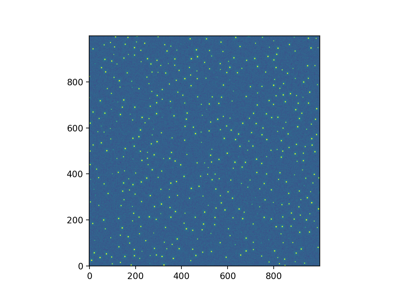
Let’s show the image:
import matplotlib.pyplot as plt
from astropy.visualization import simple_norm
from photutils.datasets import (load_simulated_hst_star_image,
                                make_noise_image)

hdu = load_simulated_hst_star_image()
data = hdu.data
data += make_noise_image(data.shape, distribution='gaussian', mean=10.0,
                         stddev=5.0, seed=123)
norm = simple_norm(data, 'sqrt', percent=99.0)
plt.imshow(data, norm=norm, origin='lower', cmap='viridis')
(Source code, png, hires.png, pdf, svg)
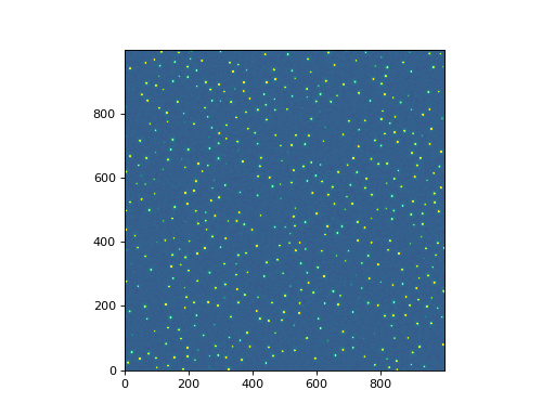
For this example we’ll use the find_peaks()
function to identify the stars and their initial positions. We will
not use the centroiding option in
find_peaks() to simulate the effect of
having imperfect initial guesses for the positions of the stars. Here we
set the detection threshold value to 500.0 to select only the brightest
stars:
>>> from photutils.detection import find_peaks
>>> peaks_tbl = find_peaks(data, threshold=500.0)
>>> peaks_tbl['peak_value'].info.format = '%.8g'  # for consistent table output
>>> print(peaks_tbl)
x_peak y_peak peak_value
------ ------ ----------
   849      2  1076.7026
   182      4  1709.5671
   324      4  3006.0086
   100      9  1142.9915
   824      9  1302.8604
   ...    ...        ...
   751    992  801.23834
   114    994  1595.2804
   299    994  648.18539
   207    998  2810.6503
   691    999  2611.0464
Length = 431 rows
Note that the stars are sufficiently separated in the simulated image that we do not need to exclude any stars due to crowding. In practice this step will require some manual inspection and selection.
Next, we need to extract cutouts of the stars using the
extract_stars() function. This function requires
a table of star positions either in pixel or sky coordinates. For
this example we are using the pixel coordinates, which need to be in
table columns called simply x and y.
We plan to extract 25 x 25 pixel cutouts of our selected stars, so let’s explicitly exclude stars that are too close to the image boundaries (because they cannot be extracted):
>>> size = 25
>>> hsize = (size - 1) / 2
>>> x = peaks_tbl['x_peak']
>>> y = peaks_tbl['y_peak']
>>> mask = ((x > hsize) & (x < (data.shape[1] -1 - hsize)) &
...         (y > hsize) & (y < (data.shape[0] -1 - hsize)))
Now let’s create the table of good star positions:
>>> from astropy.table import Table
>>> stars_tbl = Table()
>>> stars_tbl['x'] = x[mask]
>>> stars_tbl['y'] = y[mask]
The star cutouts from which we build the ePSF must have the background
subtracted. Here we’ll use the sigma-clipped median value as the
background level. If the background in the image varies across the
image, one should use more sophisticated methods (e.g.,
Background2D).
Let’s subtract the background from the image:
>>> from astropy.stats import sigma_clipped_stats
>>> mean_val, median_val, std_val = sigma_clipped_stats(data, sigma=2.0)
>>> data -= median_val
The extract_stars() function requires the input
data as an NDData object. An
NDData object is easy to create from our data
array:
>>> from astropy.nddata import NDData
>>> nddata = NDData(data=data)
We are now ready to create our star cutouts using the
extract_stars() function. For this simple
example we are extracting stars from a single image using a single
catalog. The extract_stars() can also extract
stars from multiple images using a separate catalog for each image or
a single catalog. When using a single catalog, the star positions
must be in sky coordinates (as SkyCoord
objects) and the NDData objects must contain valid
WCS objects. In the case of using multiple images
(i.e., dithered images) and a single catalog, the same physical star
will be “linked” across images, meaning it will be constrained to have
the same sky coordinate in each input image.
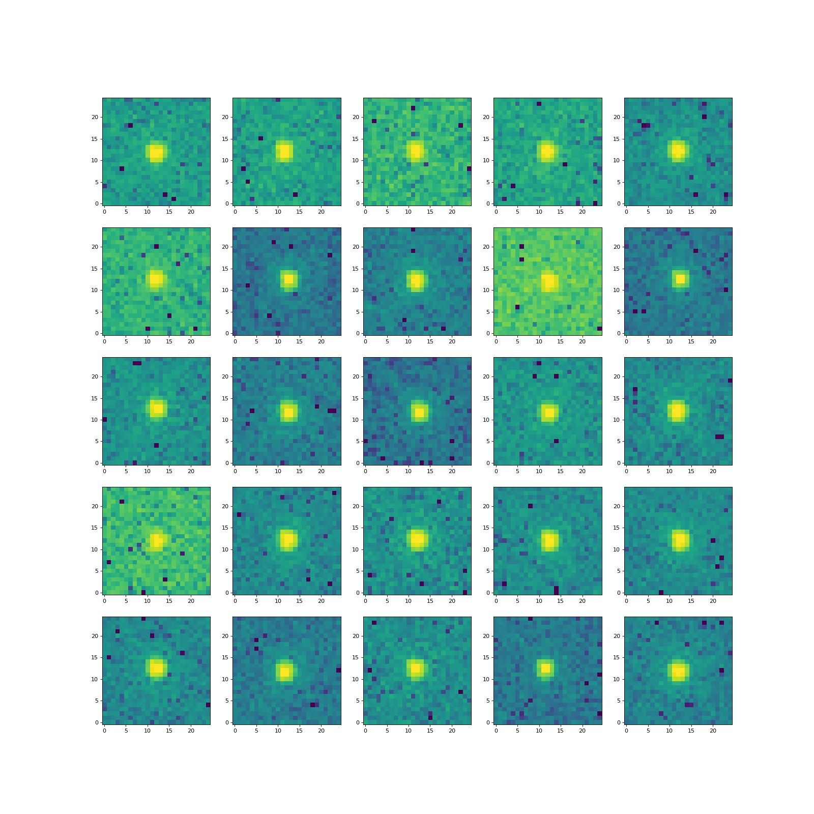
Let’s extract the 25 x 25 pixel cutouts of our selected stars:
>>> from photutils.psf import extract_stars
>>> stars = extract_stars(nddata, stars_tbl, size=25)
The function returns a EPSFStars object containing
the cutouts of our selected stars. The function extracted 403 stars,
from which we’ll build our ePSF. Let’s show the first 25 of them:
>>> import matplotlib.pyplot as plt
>>> from astropy.visualization import simple_norm
>>> nrows = 5
>>> ncols = 5
>>> fig, ax = plt.subplots(nrows=nrows, ncols=ncols, figsize=(20, 20),
...                        squeeze=True)
>>> ax = ax.ravel()
>>> for i in range(nrows * ncols):
...     norm = simple_norm(stars[i], 'log', percent=99.0)
...     ax[i].imshow(stars[i], norm=norm, origin='lower', cmap='viridis')
(Source code, png, hires.png, pdf, svg)
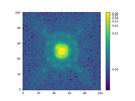
With the star cutouts in hand, we are ready to construct the ePSF with
the EPSFBuilder class. We’ll create an ePSF
with an oversampling factor of 4.0. Here we limit the maximum number of
iterations to 3 (to limit its run time), but in practice one should use
about 10 or more iterations. The EPSFBuilder
class has many other options to control the ePSF build process,
including changing the centering function, the smoothing kernel, and the
centering accuracy. Please see the EPSFBuilder
documentation for further details.
We first initialize an EPSFBuilder instance
with our desired parameters and then input the cutouts of our selected
stars to the instance:
>>> from photutils.psf import EPSFBuilder
>>> epsf_builder = EPSFBuilder(oversampling=4, maxiters=3,
...                            progress_bar=False)
>>> epsf, fitted_stars = epsf_builder(stars)
The returned values are the ePSF, as an
EPSFModel object, and our input stars fitted
with the constructed ePSF, as a new EPSFStars
object with fitted star positions and fluxes.
Finally, let’s show the constructed ePSF:
>>> import matplotlib.pyplot as plt
>>> from astropy.visualization import simple_norm
>>> norm = simple_norm(epsf.data, 'log', percent=99.0)
>>> plt.imshow(epsf.data, norm=norm, origin='lower', cmap='viridis')
>>> plt.colorbar()
(Source code, png, hires.png, pdf, svg)
The EPSFModel object is a subclass of
FittableImageModel, thus it can be used
as a PSF model for the PSF-fitting machinery in Photutils (i.e., BasicPSFPhotometry,
IterativelySubtractedPSFPhotometry, or
DAOPhotPSFPhotometry).